![]() Apr 30
Apr 30

Customer Segmentation: Excel and R
Foreward

I started reading Data Smart by John Foreman. The book is a great read because of Foreman’s humorous style of writing. What sets this book apart from the other data analysis books I have come across is that it focuses on the techniques rather than the tools – everything is accomplished through the use of a spreadsheet program (e.g. Excel).
So as a personal project to learn more about data analysis and its applications, I will be reproducing exercises in the book both in Excel and R. I will be structured in the blog posts: 0) I will always repeat this paragraph in every post 1) Introducing the Concept and Data Set, 2) Doing the Analysis with Excel, 3) Reproducing the results with R.
If you like the stuff here, please consider buying the book.
Shortcuts
This post is long, so here is a shortcut menu:
Excel
- Step 1: Pivot & Copy
- Step 2: Distances and Clusters
- Step 3: Solving for optimal cluster centers
- Step 4: Top deals by clusters
R
- Step 1: Pivot & Copy
- Step 2: Distances and Clusters
- Step 3: Solving for optimal cluster centers
- Step 4: Top deals by clusters
- Entire Code
Customer Segmentation
Customer segmentation is as simple as it sounds: grouping customers by their characteristics – and why would you want to do that? To better serve their needs!
So how does one go about segmenting customers? One method we will look at is an unsupervised method of machine learning called k-Means clustering. Unsupervised learning means finding out stuff without knowing anything about the data to start … so you want to discover.
Our example today is to do with e-mail marketing. We use the dataset from Chapter 2 on Wiley’s website – download a vanilla copy here
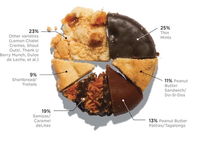
What we have are offers sent via email, and transactions based on those offers. What we want to do with K-Means clustering is classify customers based on offers they consume. Simplystatistics.org have a nice animation of what this might look like:
If we plot a given set of data by their dimensions, we can identify groups of similar points (customers) within the dataset by looking at how those points center around two or more points. The k in k-means is just the number of clusters you choose to identify; naturally this would be greater than one cluster.
Great, we’re ready to start.
K-Means Clustering – Excel
First what we need to do is create a transaction matrix. That means, we need to put the offers we mailed out next to the transaction history of each customer. This is easily achieved with a pivot table.
Step 1: Pivot & Copy
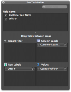 Go to your “transactions” tab and create a pivot table with the settings shown in the image to the right.
Once you have that you will have the names of the customers in columns, and the offer numbers in rows with a bunch of 1’s indicating that the customers have made a transaction based on the given offer.
Great. Copy and paste the pivot table (leaving out the grand totals column and row) into a new tab called “Matrix”.
Now copy the table from the “OfferInformation” tab and paste it to the left of your new Matrix table.
Done – You have your transaction matrix! This is what it should look like:
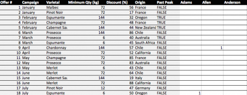
If you would like to skip this step, download this file with Step 1 completed.
Step 2: Distances and Clusters
We will use k = 4 indicating that we will use 4 clusters. This is somewhat arbitrary, but the number you pick should be representative of the number of segments you can handle as a business. So 100 segments does not make sense for an e-mail marketing campaign.
Lets go ahead and add 4 columns – each representing a cluster.
We need to calculate how far away each customer is from the cluster’s mean. To do this we could use many distances, one of which is the Euclidean Distance. This is basically the distance between two points using pythagorean theorem.
To do this in Excel we will use a feature called multi-cell arrays that will make our lives a lot easier. For “Adam” insert the following formula to calculate the distance from Cluster 1 and then press CTRL+SHIFT+ENTER (if you just press enter, Excel wont know what to do):
=SQRT(SUM((L$2:L$33-$H$2:$H$33)^2)) |
Excel will automatically add braces “{}” around your formula indicating that it will run the formula for each row.
Now do the same for clusters 2, 3 and 4.
=SQRT(SUM((L$2:L$33-$I$2:$I$33)^2)) =SQRT(SUM((L$2:L$33-$J$2:$J$33)^2)) =SQRT(SUM((L$2:L$33-$K$2:$K$33)^2)) |
Now copy Adam’s 4 cells, highlight all the “distance from cluster …” cells for the rest of the customers, and paste the formula. You now have the distances for all customers.
Before moving on we need to calculate the cluster with the minimum distance. To do this we will add 2 rows: the first is “Minimum Distance” which for Adam is:
=MIN(L34:L37) |
Do the same for the remaining customers. Then add another row labelled “Assigned Cluster” with the formula:
=MATCH(L38,L34:L37,0) |
That’s all you need. Now lets go find the optimal cluster centers!
If you would like to skip this step, download this file with Step 2 completed.
Step 3: Solving for optimal cluster centers
We will use “Solver” to help us calculate the optimal centers. This step is pretty easy now that you have most of your model set up. The optimal centers will allow us to have the minimum distance for each customer – and therefore we are minimizing the total distance.
To do this, we first must know what the total distance is. So add a row under the “Assigned Cluster” and calculate the sum of the “Minimum Distance” row using the formula:
=SUM(L38:DG38) |
We are now ready to use solver (found in Tools -> Solver). Set up your solver to match the following screenshot.
Note that we change the solver to “evolutionary” and set options of convergence to 0.00001, and timeout to 600 seconds.

When ready, press solve. Go make yourself a coffee, this will take about 10 minutes.
Note: Foreman is able to achieve 140, I only reached 144 before my computer times out. This is largely due to my laptop’s processing power I believe. Nevertheless, the solution is largely acceptable.
I think it’s a good time to appropriately name your tab “Clusters”.
If you would like to skip this step, download this file with Step 3 completed.
Step 4: Top deals by clusters
Now we have our clusters – and essentially our segments – we want to find the top deals for each segment. That means we want to calculate, for each offer, how many were consumed by each segment.
This is easily achieved through the SUMIF function in excel. First lets set up a new tab called “Top Deals”. Copy and paste the “Offer Information” tab into your new Top Deals tab and add 4 empty columns labelled 1,2,3, and 4.
The SUMIF formula uses 3 arguments: the data you want to consider, the criteria whilst considering that data, and finally if the criteria is met what should the formula sum up. In our case we will consider the clusters as the data, the cluster number as the criteria, and the number of transactions for every offer as the final argument.
This is done using the following formula in the cell H2 (Offer 1, Cluster 1):
=SUMIF(Clusters!$L$39:$DG$39,'Top Deals'!H$1,Clusters!$L2:$DG2) |
Drag this across (or copy and paste into) cells H2 to K33. You now have your top deals! It’s not very clear though so add some conditional formatting by highlighting H2:K33 and selecting format -> conditional formatting. I added the following rule:
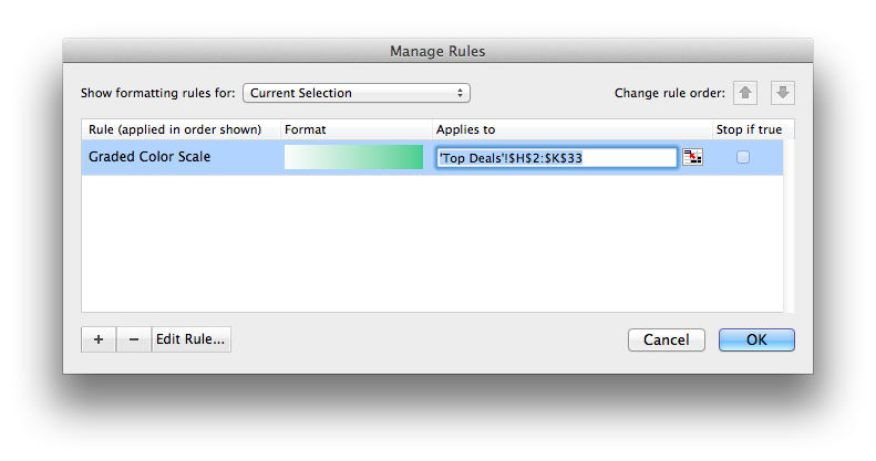
That’s it! Foreman goes into details about how to judge whether 4 clusters are enough but this is beyond the scope of the post. We have 4 clusters and our offers assigned to each cluster. The rest is interpretation. One observation that stands out is that cluster 4 was the only cluster that consumed Offer 22.
Another is that cluster 1 have clear preferences for Pinot Noir offers and so we will push Pinot Noir offers to: Anderson, Bell, Campbell, Cook, Cox, Flores, Jenkins, Johnson, Moore, Morris, Phillips, Smith. You could even use a cosine similarity or apriori recommendations to go a step further with Cluster 1.
We are done with Excel, now lets see how to do this with R!
If you would like to skip this step, download this file with Step 4 completed.
K-Means Clustering – R
We will go through the same steps we did. We start with our vanilla files – provided in CSV format:
Download these files into a folder where you will work from in R. Fire up RStudio and lets get started.
Step 1: Pivot & Copy
First we want to read our data. This is simple enough:
# Read offers and transaction data offers<-read.csv(file="OfferInformation.csv") transactions<-read.csv(file="Transactions.csv") |
We now need to combine these 2 files to get a frequency matrix – equivalent to pivoting in Excel. This can be done using the reshape library in R. Specifically we will use the melt and cast functions.
We first melt the 2 columns of the transaction data. This will create data that we can pivot: customer, variable, and value. We only have 1 variable here – Offer.
We then want to cast this data by putting value first (the offer number) in rows, customer names in the columns. This is done by using R’s style of formula input: Value ~ Customers.
We then want to count each occurrence of customers in the row. This can be done by using a function that takes customer names as input, counts how many there are, and returns the result. Simply: function(x) length(x)
Lastly, we want to combine the data from offers with our new transaction matrix. This is done using cbind (column bind) which glues stuff together automagically.
Lots of explanations for 3 lines of code!
#Load Library library(reshape) # Melt transactions, cast offer by customers pivot<-melt(transactions[1:2]) pivot<-(cast(pivot,value~Customer.Last.Name,fill=0,fun.aggregate=function(x) length(x))) # Bind to offers, we remove the first column of our new pivot because it's redundant. pivot<-cbind(offers,pivot[-1]) |
We can output the pivot table into a new CSV file called pivot.
write.csv(file="pivot.csv",pivot)
Step 2: Clustering
To cluster the data we will use only the columns starting from “Adams” until “Young”.
We will use the fpc library to run the KMeans algorithm with 4 clusters.
To use the algorithm we will need to rotate the transaction matrix with t().
That’s all you need: 4 lines of code!
# Load library library(fpc) # Only use customer transaction data and we will rotate the matrix cluster.data<-pivot[,8:length(pivot)] cluster.data<-t(cluster.data) # We will run KMeans using pamk (more robust) with 4 clusters. cluster.kmeans<-pamk(cluster.data,k=4) # Use this to view the clusters View(cluster.kmeans$pamobject$clustering) |
Step 3: Solving for Cluster Centers
This is not a necessary step in R! Pat yourself on the back, get another cup of tea or coffee and move onto to step 4.
Step 4: Top deals by clusters
Top get the top deals we will have to do a little bit of data manipulation. First we need to combine our clusters and transactions. Noteably the lengths of the ‘tables’ holding transactions and clusters are different. So we need a way to merge the data … so we use the merge() function and give our columns sensible names:
#Merge Data cluster.deals<-merge(transactions[1:2],cluster.kmeans$pamobject$clustering,by.x = "Customer.Last.Name", by.y = "row.names") colnames(cluster.deals)<-c("Name","Offer","Cluster") |
We then want to repeat the pivoting process to get Offers in rows and clusters in columns counting the total number of transactions for each cluster. Once we have our pivot table we will merge it with the offers data table like we did before:
# Melt, cast, and bind cluster.pivot<-melt(cluster.deals,id=c("Offer","Cluster")) cluster.pivot<-cast(cluster.pivot,Offer~Cluster,fun.aggregate=length) cluster.topDeals<-cbind(offers,cluster.pivot[-1]) |
We can then reproduce the excel version by writing to a csv file:
write.csv(file="topdeals.csv",cluster.topDeals,row.names=F) |
Note
It’s important to note that cluster 1 in excel does not correspond to cluster 1 in R. It’s just the way the algorithms run. Moreover, the allocation of clusters might differ slightly because of the nature of kmeans algorithm. However, your insights will be the same; in R we also see that cluster 3 prefers Pinot Noir and cluster 4 has a strong preference for Offer 22.
Entire Code
# Read data offers<-read.csv(file="OfferInformation.csv") transactions<-read.csv(file="Transactions.csv") # Create transaction matrix library(reshape) pivot<-melt(transactions[1:2]) pivot<-(cast(pivot,value~Customer.Last.Name,fill=0,fun.aggregate=function(x) length(x))) pivot<-cbind(offers,pivot[-1]) write.csv(file="pivot.csv",pivot) # Cluster library(fpc) cluster.data<-pivot[,8:length(pivot)] cluster.data<-t(cluster.data) cluster.kmeans<-pamk(cluster.data,k=4) # Merge Data cluster.deals<-merge(transactions[1:2],cluster.kmeans$pamobject$clustering,by.x = "Customer.Last.Name", by.y = "row.names") colnames(cluster.deals)<-c("Name","Offer","Cluster") # Get top deals by cluster cluster.pivot<-melt(cluster.deals,id=c("Offer","Cluster")) cluster.pivot<-cast(cluster.pivot,Offer~Cluster,fun.aggregate=length) cluster.topDeals<-cbind(offers,cluster.pivot[-1]) write.csv(file="topdeals.csv",cluster.topDeals,row.names=F) |
![]() Posted by Salem
Posted by Salem
![]() Apr 26
Apr 26

Collaborative Filtering with R
We already looked at Market Basket Analysis with R. Collaborative filtering is another technique that can be used for recommendation.
The underlying concept behind this technique is as follows:
- Assume Person A likes Oranges, and Person B likes Oranges.
- Assume Person A likes Apples.
- Person B is likely to have similar opinions on Apples as A than some other random person.
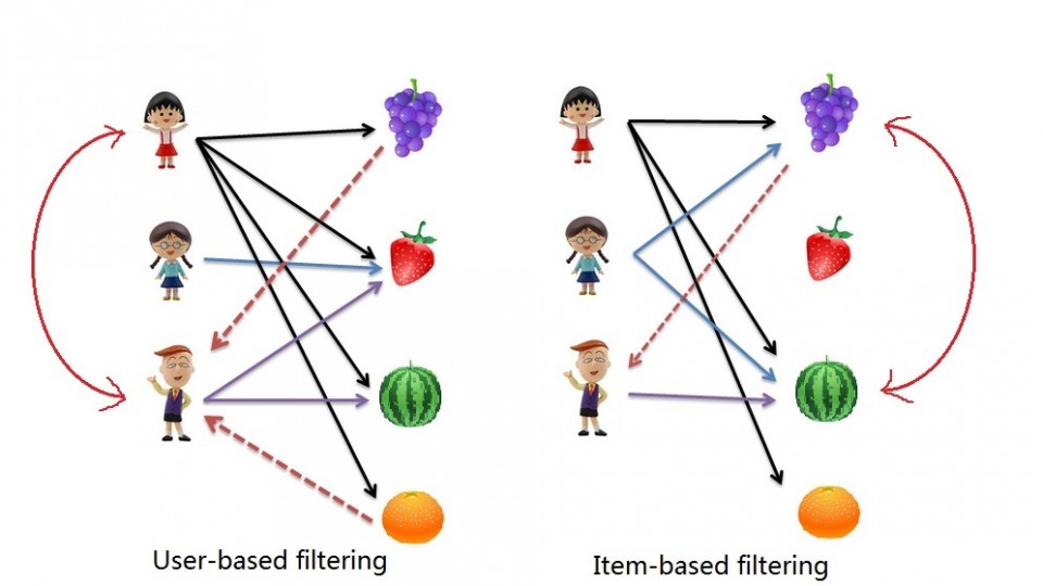
The implications of collaborative filtering are obvious: you can predict and recommend items to users based on preference similarities. There are two types of collaborative filtering: user-based and item-based.
Item Based Collaborative Filtering takes the similarities between items’ consumption history.
User Based Collaborative Filtering considers similarities between user consumption history.
We will look at both types of collaborative filtering using a publicly available dataset from LastFM.
Case: Last.FM Music
The data set contains information about users, their gender, their age, and which artists they have listened to on Last.FM. We will not use the entire dataset. For simplicity’s sake we only use songs in Germany and we will transform the data to a item frequency matrix. This means each row will represent a user, and each column represents and artist. For this we use R’s “reshape” package. This is largely administrative, so we will start with the transformed dataset.
Download the LastFM Germany frequency matrix and put it in your working directory. Load up R and read the data file.
# Read data from Last.FM frequency matrix data.germany <- read.csv(file="lastfm-matrix-germany.csv") |
Lets look at a sample of our data. The output looks something like this:
head(data.germany[,c(1,3:8)]) user abba ac.dc adam.green aerosmith afi air 1 1 0 0 0 0 0 0 2 33 0 0 1 0 0 0 3 42 0 0 0 0 0 0 4 51 0 0 0 0 0 0 5 62 0 0 0 0 0 0 6 75 0 0 0 0 0 0 |
We’re good to go!
Item Based Collaborative Filtering
In item based collaborative filtering we do not really care about the users. So the first thing we should do is drop the user column from our data. This is really easy since it is the first column, but if it was not the first column we would still be able to drop it with the following code:
# Drop any column named "user" data.germany.ibs <- (data.germany[,!(names(data.germany) %in% c("user"))]) |
We then want to calculate the similarity of each song with the rest of the songs. This means that we want to compare each column in our “data.germany.ibs” data set with every other column in the data set. Specifically, we will be comparing what is known as the “Cosine Similarity”.
The cosine similarity, in essence takes the sum product of the first and second column, and divide that by the product of the square root of the sum of squares of each column. (that was a mouth-full!)
The important thing to know is the resulting number represents how “similar” the first column is with the second column. We will use the following helper function to product the Cosine Similarity:
# Create a helper function to calculate the cosine between two vectors getCosine <- function(x,y) { this.cosine <- sum(x*y) / (sqrt(sum(x*x)) * sqrt(sum(y*y))) return(this.cosine) } |
We are now ready to start comparing each of our songs (items). We first need a placeholder to store the results of our cosine similarities. This placeholder will have the songs in both columns and rows:
# Create a placeholder dataframe listing item vs. item data.germany.ibs.similarity <- matrix(NA, nrow=ncol(data.germany.ibs),ncol=ncol(data.germany.ibs),dimnames=list(colnames(data.germany.ibs),colnames(data.germany.ibs))) |
The first 6 items of the empty placeholder will look like this:
a.perfect.circle abba ac.dc adam.green aerosmith afi a.perfect.circle NA NA NA NA NA NA abba NA NA NA NA NA NA ac.dc NA NA NA NA NA NA adam.green NA NA NA NA NA NA aerosmith NA NA NA NA NA NA afi NA NA NA NA NA NA |
Perfect, all that’s left is to loop column by column and calculate the cosine similarities with our helper function, and then put the results into the placeholder data table. That sounds like a pretty straight-forward nested for-loop:
# Lets fill in those empty spaces with cosine similarities # Loop through the columns for(i in 1:ncol(data.germany.ibs)) { # Loop through the columns for each column for(j in 1:ncol(data.germany.ibs)) { # Fill in placeholder with cosine similarities data.germany.ibs.similarity[i,j] <- getCosine(as.matrix(data.germany.ibs[i]),as.matrix(data.germany.ibs[j])) } } # Back to dataframe data.germany.ibs.similarity <- as.data.frame(data.germany.ibs.similarity) |
Note: For loops in R are infernally slow. We use as.matrix() to transform the columns into matrices since matrix operations run a lot faster. We transform the similarity matrix into a data.frame for later processes that we will use.
We have our similarity matrix. Now the question is … so what?
We are now in a position to make recommendations! We look at the top 10 neighbours of each song – those would be the recommendations we make to people listening to those songs.
We start off by creating a placeholder:
# Get the top 10 neighbours for each data.germany.neighbours <- matrix(NA, nrow=ncol(data.germany.ibs.similarity),ncol=11,dimnames=list(colnames(data.germany.ibs.similarity))) |
Our empty placeholder should look like this:
[,1] [,2] [,3] [,4] [,5] [,6] [,7] [,8] [,9] [,10] [,11] a.perfect.circle NA NA NA NA NA NA NA NA NA NA NA abba NA NA NA NA NA NA NA NA NA NA NA ac.dc NA NA NA NA NA NA NA NA NA NA NA adam.green NA NA NA NA NA NA NA NA NA NA NA aerosmith NA NA NA NA NA NA NA NA NA NA NA afi NA NA NA NA NA NA NA NA NA NA NA |
Then we need to find the neighbours. This is another loop but runs much faster.
for(i in 1:ncol(data.germany.ibs)) { data.germany.neighbours[i,] <- (t(head(n=11,rownames(data.germany.ibs.similarity[order(data.germany.ibs.similarity[,i],decreasing=TRUE),][i])))) } |
It’s a little bit more complicated so lets break it down into steps:
- We loop through all our artists
- We sort our similarity matrix for the artist so that we have the most similar first.
- We take the top 11 (first will always be the same artist) and put them into our placeholder
- Note we use t() to rotate the similarity matrix since the neighbour one is shaped differently
The filled in placeholder should look like this:
[,1] [,2] [,3] a.perfect.circle "a.perfect.circle" "tool" "dredg" abba "abba" "madonna" "robbie.williams" ac.dc "ac.dc" "red.hot.chilli.peppers" "metallica" adam.green "adam.green" "the.libertines" "the.strokes" aerosmith "aerosmith" "u2" "led.zeppelin" afi "afi" "funeral.for.a.friend" "rise.against" |
This means for those listening to Abba we would recommend Madonna and Robbie Williams.
Likewise for people listening to ACDC we would recommend the Red Hot Chilli Peppers and Metallica.
User Based Recommendations
We will need our similarity matrix for User Based recommendations.
The process behind creating a score matrix for the User Based recommendations is pretty straight forward:
- Choose an item and check if a user consumed that item
- Get the similarities of that item’s top X neighbours
- Get the consumption record of the user of the top X neighbours
- Calculate the score with a formula: sumproduct(purchaseHistory, similarities)/sum(similarities)
We can start by creating a helper function to calculate the score mentioned in the last step.
# Lets make a helper function to calculate the scores getScore <- function(history, similarities) { x <- sum(history*similarities)/sum(similarities) x } |
We will also need a holder matrix. We will use the original data set now (data.germany):
# A placeholder matrix holder <- matrix(NA, nrow=nrow(data.germany),ncol=ncol(data.germany)-1,dimnames=list((data.germany$user),colnames(data.germany[-1]))) |
The rest is one big ugly nested loop. First the loop, then we will break it down step by step:
# Loop through the users (rows) for(i in 1:nrow(holder)) { # Loops through the products (columns) for(j in 1:ncol(holder)) { # Get the user's name and th product's name # We do this not to conform with vectors sorted differently user <- rownames(holder)[i] product <- colnames(holder)[j] # We do not want to recommend products you have already consumed # If you have already consumed it, we store an empty string if(as.integer(data.germany[data.germany$user==user,product]) == 1) { holder[i,j]<-"" } else { # We first have to get a product's top 10 neighbours sorted by similarity topN<-((head(n=11,(data.germany.ibs.similarity[order(data.germany.ibs.similarity[,product],decreasing=TRUE),][product])))) topN.names <- as.character(rownames(topN)) topN.similarities <- as.numeric(topN[,1]) # Drop the first one because it will always be the same song topN.similarities<-topN.similarities[-1] topN.names<-topN.names[-1] # We then get the user's purchase history for those 10 items topN.purchases<- data.germany[,c("user",topN.names)] topN.userPurchases<-topN.purchases[topN.purchases$user==user,] topN.userPurchases <- as.numeric(topN.userPurchases[!(names(topN.userPurchases) %in% c("user"))]) # We then calculate the score for that product and that user holder[i,j]<-getScore(similarities=topN.similarities,history=topN.userPurchases) } # close else statement } # end product for loop } # end user for loop data.germany.user.scores <- holder |
The loop starts by taking each user (row) and then jumps into another loop that takes each column (artists).
We then store the user’s name and artist name in variables to use them easily later.
We then use an if statement to filter out artists that a user has already listened to – this is a business case decision.
The next bit gets the item based similarity scores for the artist under consideration.
# We first have to get a product's top 10 neighbours sorted by similarity topN<-((head(n=11,(data.germany.ibs.similarity[order(data.germany.ibs.similarity[,product],decreasing=TRUE),][product])))) topN.names <- as.character(rownames(topN)) topN.similarities <- as.numeric(topN[,1]) # Drop the first one because it will always be the same song topN.similarities<-topN.similarities[-1] topN.names<-topN.names[-1] |
It is important to note the number of artists you pick matters. We pick the top 10.
We store the similarities score and song names.
We also drop the first column because, as we saw, it always represents the same song.
We’re almost there. We just need the user’s purchase history for the top 10 songs.
# We then get the user's purchase history for those 10 items topN.purchases<- data.germany[,c("user",topN.names)] topN.userPurchases<-topN.purchases[topN.purchases$user==user,] topN.userPurchases <- as.numeric(topN.userPurchases[!(names(topN.userPurchases) %in% c("user"))]) |
We use the original data set to get the purchases of our users’ top 10 purchases.
We filter out our current user in the loop and then filter out purchases that match the user.
We are now ready to calculate the score and store it in our holder matrix:
# We then calculate the score for that product and that user holder[i,j]<-getScore(similarities=topN.similarities,history=topN.userPurchases) |
Once we are done we can store the results in a data frame.
The results should look something like this:
X a.perfect.circle abba ac.dc 1 0.0000000 0.00000000 0.20440540 33 0.0823426 0.00000000 0.09591153 42 0.0000000 0.08976655 0.00000000 51 0.0823426 0.08356811 0.00000000 62 0.0000000 0.00000000 0.11430459 75 0.0000000 0.00000000 0.00000000 |
This basically reads that for user 51 we would recommend abba first, then a perfect circle, and we would not recommend ACDC.
This is not very pretty … so lets make it pretty:
We will create another holder matrix and for each user score we will sort the scores and store the artist names in rank order.
# Lets make our recommendations pretty data.germany.user.scores.holder <- matrix(NA, nrow=nrow(data.germany.user.scores),ncol=100,dimnames=list(rownames(data.germany.user.scores))) for(i in 1:nrow(data.germany.user.scores)) { data.germany.user.scores.holder[i,] <- names(head(n=100,(data.germany.user.scores[,order(data.germany.user.scores[i,],decreasing=TRUE)])[i,])) } |
The output of this will look like this:
X V1 V2 V3 1 flogging.molly coldplay aerosmith 33 peter.fox gentleman red.hot.chili.peppers 42 oomph. lacuna.coil rammstein 51 the.subways the.kooks the.hives 62 mando.diao the.fratellis jack.johnson 75 hoobastank papa.roach the.prodigy |
By sorting we see that actually the top 3 for user 51 is the subways, the kooks, and the hives!
References
- Data Mining and Business Analytics with R
- This case is based on Professor Miguel Canela “Designing a music recommendation app”
Entire Code
# Admin stuff here, nothing special options(digits=4) data <- read.csv(file="lastfm-data.csv") data.germany <- read.csv(file="lastfm-matrix-germany.csv") ############################ # Item Based Similarity # ############################ # Drop the user column and make a new data frame data.germany.ibs <- (data.germany[,!(names(data.germany) %in% c("user"))]) # Create a helper function to calculate the cosine between two vectors getCosine <- function(x,y) { this.cosine <- sum(x*y) / (sqrt(sum(x*x)) * sqrt(sum(y*y))) return(this.cosine) } # Create a placeholder dataframe listing item vs. item holder <- matrix(NA, nrow=ncol(data.germany.ibs),ncol=ncol(data.germany.ibs),dimnames=list(colnames(data.germany.ibs),colnames(data.germany.ibs))) data.germany.ibs.similarity <- as.data.frame(holder) # Lets fill in those empty spaces with cosine similarities for(i in 1:ncol(data.germany.ibs)) { for(j in 1:ncol(data.germany.ibs)) { data.germany.ibs.similarity[i,j]= getCosine(data.germany.ibs[i],data.germany.ibs[j]) } } # Output similarity results to a file write.csv(data.germany.ibs.similarity,file="final-germany-similarity.csv") # Get the top 10 neighbours for each data.germany.neighbours <- matrix(NA, nrow=ncol(data.germany.ibs.similarity),ncol=11,dimnames=list(colnames(data.germany.ibs.similarity))) for(i in 1:ncol(data.germany.ibs)) { data.germany.neighbours[i,] <- (t(head(n=11,rownames(data.germany.ibs.similarity[order(data.germany.ibs.similarity[,i],decreasing=TRUE),][i])))) } # Output neighbour results to a file write.csv(file="final-germany-item-neighbours.csv",x=data.germany.neighbours[,-1]) ############################ # User Scores Matrix # ############################ # Process: # Choose a product, see if the user purchased a product # Get the similarities of that product's top 10 neighbours # Get the purchase record of that user of the top 10 neighbours # Do the formula: sumproduct(purchaseHistory, similarities)/sum(similarities) # Lets make a helper function to calculate the scores getScore <- function(history, similarities) { x <- sum(history*similarities)/sum(similarities) x } # A placeholder matrix holder <- matrix(NA, nrow=nrow(data.germany),ncol=ncol(data.germany)-1,dimnames=list((data.germany$user),colnames(data.germany[-1]))) # Loop through the users (rows) for(i in 1:nrow(holder)) { # Loops through the products (columns) for(j in 1:ncol(holder)) { # Get the user's name and th product's name # We do this not to conform with vectors sorted differently user <- rownames(holder)[i] product <- colnames(holder)[j] # We do not want to recommend products you have already consumed # If you have already consumed it, we store an empty string if(as.integer(data.germany[data.germany$user==user,product]) == 1) { holder[i,j]<-"" } else { # We first have to get a product's top 10 neighbours sorted by similarity topN<-((head(n=11,(data.germany.ibs.similarity[order(data.germany.ibs.similarity[,product],decreasing=TRUE),][product])))) topN.names <- as.character(rownames(topN)) topN.similarities <- as.numeric(topN[,1]) # Drop the first one because it will always be the same song topN.similarities<-topN.similarities[-1] topN.names<-topN.names[-1] # We then get the user's purchase history for those 10 items topN.purchases<- data.germany[,c("user",topN.names)] topN.userPurchases<-topN.purchases[topN.purchases$user==user,] topN.userPurchases <- as.numeric(topN.userPurchases[!(names(topN.userPurchases) %in% c("user"))]) # We then calculate the score for that product and that user holder[i,j]<-getScore(similarities=topN.similarities,history=topN.userPurchases) } # close else statement } # end product for loop } # end user for loop # Output the results to a file data.germany.user.scores <- holder write.csv(file="final-user-scores.csv",data.germany.user.scores) # Lets make our recommendations pretty data.germany.user.scores.holder <- matrix(NA, nrow=nrow(data.germany.user.scores),ncol=100,dimnames=list(rownames(data.germany.user.scores))) for(i in 1:nrow(data.germany.user.scores)) { data.germany.user.scores.holder[i,] <- names(head(n=100,(data.germany.user.scores[,order(data.germany.user.scores[i,],decreasing=TRUE)])[i,])) } # Write output to file write.csv(file="final-user-recommendations.csv",data.germany.user.scores.holder) |
![]() Posted by Salem
Posted by Salem
![]() Apr 7
Apr 7

Kuwait Stock Exchange P/E with R
Foreword
I was inspired by Meet Saptarsi’s post on R-Bloggers.com and decided to emulate the process for the Kuwait Stock Exchange.
Disclaimer This is not financial advice of any sort! I did this to demonstrate how R can be used to scrape information about the Kuwait Stock Exchange listed companies and do basic data analysis on the data.
Dig in!
First we want to set up the libraries we will use in our script.
We will be using XML to scrape websites and GGPlot2 to create our graphs.
library(XML) library('ggplot2') |
Kuwait Stock Exchange – Ticker Symbols
Initially I thought we could get all the information we want from the Kuwait stock exchange (KSE) website. I was terribly mistaken. KSE.com.kw is so behind the times … but atleast we can accurately gather the ticker names of companies listed in the KSE.
The process is simple.
- Find the page with information you want: http://www.kuwaitse.com/Stock/Companies.aspx
- Use readHTMLTable() to read the page, and find a table. In this case it’s table #35
- Now you have a data frame that you can access the tickers!
# Read Stock Information from KSE kse.url <- "http://www.kuwaitse.com/Stock/Companies.aspx" tables <- readHTMLTable(kse.url,head=T,which=35) tickers<-tables$Ticker |
P/E Ratios
P/E ratios are used to guage growth expectations of a company compared to others within a sector. You can find details about the P/E ratio here, but we will suffice by saying that we want to know what the market looks like in terms of P/E ratios.
Ideally the P/E ratio would be available from KSE or atleast access to digital forms of each company's financial statements. I was unable to find such a thing so I turned to MarketWatch.com. We can use the ticker codes we collected to grab the data we need.
The process is different because MarketWatch does not have HTML tables. Instead the process is slightly more complicated.
- Create a holder data frame
- Loop through each ticker and point to the relevant page:
http://www.marketwatch.com/investing/Stock/TICKER-NAME?countrycode=KW
Replacing TICKER-NAME with the ticker name - We go through the HTML elements of the page until we find the P/E Ratio
- Once we have collected all the P/E ratios, we do some data cleaning and we’re done!
What’s interesting is that after the data cleansing we lose 40 odd companies because there is no data available on their P/E ratios. This could also mean that these companies are losing money … because companies with no earnings have no P/E ratio! Realistically this is not a large number to hunt for but we omit them for the sake of simplicity here.
# Create an empty frame first pe.data <- data.frame('Ticker'='','PE'='') pe.data <- pe.data[-1,] # Loop through the ticker symbols for(i in 1:length(tickers)) { this.ticker<-tickers[i] # Set up the URL to use this.url <- paste("http://www.marketwatch.com/investing/Stock/",tickers[i],"?countrycode=KW",sep="") # Get the page source this.doc <- htmlTreeParse(this.url, useInternalNodes = T) # We can look at the HTML parts that contain the PE ratio this.nodes<-getNodeSet(this.doc, "//div[@class='section']//p") # We look for the value of the PE ratio within the nodes this.pe<-suppressWarnings(as.numeric(sapply(this.nodes[4], xmlValue,'data'))) # Add a row to the P/E data frame and move onto the next ticker! symbol pe.data<-rbind(pe.data,data.frame('Ticker'=this.ticker,'PE'=this.pe)) } # Combine the P/E data frame with the KSE ticker data frame combined<-(cbind(tables,pe.data)) # Lets do some data cleaning removing the 'NAs' combined.clean<-(combined[!(combined$PE %in% NA),]) # We attach our data frame to use the names of columns as variables attach(combined.clean) |
Data Exploration
We draw a box plot and output summary statistics.
We see that we have a number of outliers and generally the majority of P/E ratios are centered around 20.94.
boxplot(PE,col='blue') summary(PE) |
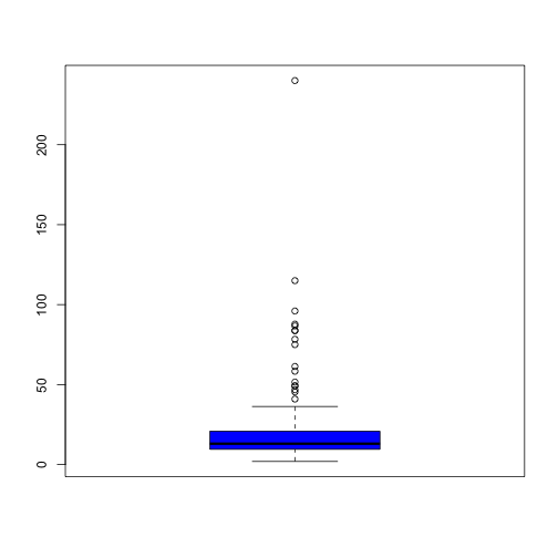
## Min. 1st Qu. Median Mean 3rd Qu. Max. ## 1.93 9.55 13.00 20.90 20.80 240.00 |
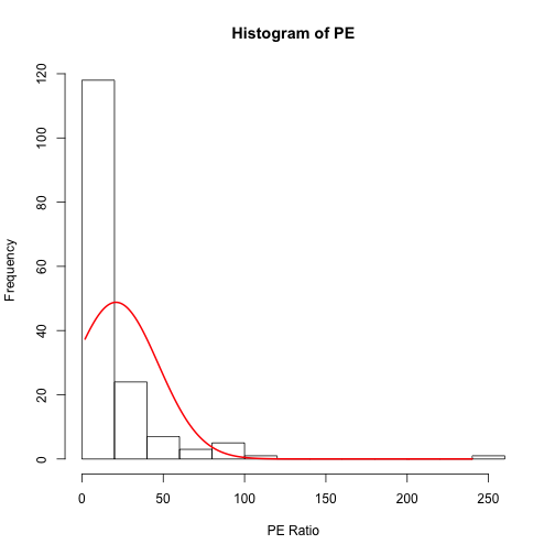
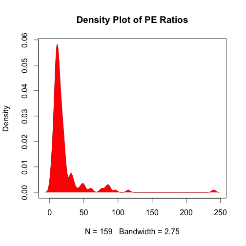
To see the spread we can look at a histogram or a density plot.
Both plots confirm a strong skew in the PE ratios.
# We can make a histogram histogram<-hist(PE,xlab="PE Ratio") # Draw a normal curve xfit<-seq(min(PE),max(PE)) yfit<-dnorm(xfit,mean=mean(PE),sd=sd(PE)) yfit <- yfit*diff(histogram$mids[1:2])*length(PE) lines(xfit, yfit, col="red", lwd=2) |
# Alternatively we can use a density plot plot(density(PE),main="Density Play of PE Ratios") polygon(density(PE), col="red", border="red",lwd=1) |
Scatter plot by industry
Lets get with it then.
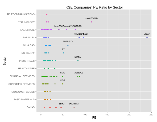
We want to see a plot of the P/E ratios by industry.
# We will want to highlihgt the outliers so lets get the outliers from our box plot outliers<-combined.clean[(which(PE %in% (boxplot.stats(PE)$out))),] # Lets create a Scatter Plot highlighting our outliers qplot(PE,Sector,main="KSE Companies' PE Ratio by Sector") + geom_point(aes(colour=Sector)) + geom_text(data=outliers,aes(label=outliers$Ticker),vjust=-2,cex=3)+ theme(legend.position = "none") |

We can clearly see the outliers. Generally outliers should tell you that something is fundamentally wrong. A company with a super high P/E ratio compared to its peers means that they have had terrible earnings, that investor expect some sort of extraordinary performance irrespective of the price, or that there is something fundamentally questionable about the numbers and you should dig in deeper. For details you can check out Investopedia.com
# Lets print out the outlier names (data.frame(outliers$Sector,outliers$Name)) |
## outliers.Sector outliers.Name ## 1 OIL & GAS THE ENERGY HOUSE CO ## 2 INDUSTRIALS NATIONAL INDUSTRIES COMPANY ## 3 CONSUMER SERVICES UNITED FOODSTUFF INDUSTRIES GROUP CO. ## 4 BANKS COMMERCIAL BANK OF KUWAIT ## 5 BANKS BURGAN BANK ## 6 BANKS BOUBYAN BANK ## 7 INSURANCE FIRST TAKAFUL INSURANCE COMPANY ## 8 REAL ESTATE INJAZZAT REAL ESTATE DEV. CO ## 9 REAL ESTATE INVESTORS HOLDING GROUP CO. ## 10 REAL ESTATE SANAM REAL ESTATE CO. ## 11 FINANCIAL SERVICES FIRST INVESTMENT COMPANY ## 12 FINANCIAL SERVICES OSOUL INVESTMENT CO. ## 13 FINANCIAL SERVICES KUWAIT CHINA INVESTMENT COMPANY ## 14 TECHNOLOGY HAYAT COMMUNICATIONS COMPANY ## 15 PARALLEL AL-BAREEQ HOLDING CO. ## 16 PARALLEL AL-MAIDAN CLINIC FOR ORAL HEALTH SERVICES CO. ## 17 PARALLEL DAR AL THURAYA REAL ESTATE CO. |
![]() Posted by Salem
Posted by Salem


Chatter