![]() May 4
May 4
Tweet Bayes Classification: Excel and R

Foreward

I started reading Data Smart by John Foreman. The book is a great read because of Foreman’s humorous style of writing. What sets this book apart from the other data analysis books I have come across is that it focuses on the techniques rather than the tools – everything is accomplished through the use of a spreadsheet program (e.g. Excel).
So as a personal project to learn more about data analysis and its applications, I will be reproducing exercises in the book both in Excel and R. I will be structured in the blog posts: 0) I will always repeat this paragraph in every post 1) Introducing the Concept and Data Set, 2) Doing the Analysis with Excel, 3) Reproducing the results with R.
If you like the stuff here, please consider buying the book.
Shortcuts
This post is long, so here is a shortcut menu:
http___www.bigleaguekickball.com_category_press_ SOMA OVERNIGHT COD Excel
- Step 1: Data Cleaning
- Step 2: Word Counting
- Step 3: Tokenization
- Step 4: Model Building
- Step 5: Using Bayes and the MAP model
http___www.bigleaguekickball.com_about_ Soma online ordering next day VISA Mastercard accepted R
- Step 1: Data Cleaning
- Step 2: Word Counting
- Step 3: Tokenization
- Step 4: Model Building
- Step 5: Using Bayes and the MAP model
- Entire Code
Tweet Classification
The problem we are going to tackle here is one of classification. We want to know if blocks of texts can be classified into groups based on some model that we build. Specifically we are going to work with a small data set of tweets that have been pre-classified to make a model that will classify new tweets that we have not seen before.
We will be using a Naïve Bayes Classification model. This technique is useful not just for tweets, it can be used for any type of natural language classification: for example e-mail/sms spam filters, loan application risk screening, blog domain classification.
 The case is about Mandrill.com who are monitoring tweets with the tag “Mandrill”. We want to be able to classify tweets automagically into two categories: “relevant” and “irrelevant”.
The problem is that Mandrill is not necessarily a unique word. I searched Twitter for Mandrill and I get 5 tweets that are relevant, and 2 that are not … and the rest do not fit in my screenshot. There are many irrelevant ones beyond that … so do we just get trolled by the rest of the mandrill tweets?
Nope! Lets get started.
Download the vanilla excel files here:
Mandrill – Vanilla
Tweet Classification with Naive Bayes Classifier: Excel
In your Excel file you will have 3 tabs each containing tweets. The first tab contains 150 relevant tweets, the second tab labeled “AboutOther” contains irrelevant tweets, and the last tab has tweets we will use to test the model we are about to develop.
Step 1: Data Cleaning
We will need to do the following for data in the first two tabs. Repeat everything in step 1 for the “AboutMandrilApp” and “AboutOther” tabs.
The first thing we need to do is make everything in non-capital letters. This is done by using the lower() formula. Let us place the formula in cell B2 and drag the formula down to cell B151.
=lower(A2) |
Next we need to swap punctuation with spaces. Specifically we swap these characters with spaces: “. “, “: “, “?”, “!”, “;”, “,”. Note the space after the full-stop and the colon is important. We need to add six columns in each tab use the substitute() function. Place the following 6 in cells C2,D2,E2,F2,G2 and drag them down to row 151:
=SUBSTITUTE(B2,". "," ") =SUBSTITUTE(C2,": "," ") =SUBSTITUTE(D2,"?"," ") =SUBSTITUTE(E2,"!"," ") =SUBSTITUTE(F2,";"," ") =SUBSTITUTE(G2,","," ") |
You can skip this step by downloading the file with this step completed: Mandrill – Step 1
Step 2: Word Counting
Tokenization just means splitting up our sentences (in this case tweets) word by word. Naturally words are split by spaces so we will be using ” ” to split our words. The goal is to have a list of all the words separately in a list. This means we need to figure out how many words we have per tweet to understand how many rows we will need.
We can count the number of words per line by counting the number of spaces in a sentence and adding 1. For example: “The red fox runs fast” has 4 spaces and 5 words. To count spaces we need to subtract the number of characters in a sentence with spaces from the number of characters in the same sentence without spaces. In our example, that would be 21 – 17 which is 4 spaces … and therefore 5 words! This is easily achieved with the following formula copied into column i:
=IF(LEN(TRIM(H2))=0,0,LEN(TRIM(H2))-LEN(SUBSTITUTE(H2," ",""))+1) |
We then see that the maximum number of words is 28 … so we will be safe and take 30 words per sentence. We have 150 tweets, and 30 words per tweet, so we will need 4500 rows for all the words.
Great! We need 2 new tabs now: one called MandrillTokens and the other OtherTokens. Label cell A1 in each of these tabs “Tweet”. Next, copy cell H2 from the MandrillApp tab. Highlight cells A2 to A4501 in the MandrillTokens tab and paste only the values into the cells. This can be accomplished by using the Paste Special option in the Edit menu. You will notice that the tweets will repeat after row 151, this is good since we need to use the same tweet at least 30 times. Repeat this for OtherTokens.
We are now ready to Tokenize! (Wohoo!!)
You can skip this step by downloading the file with this step completed: Mandrill – Step 2
Step 3: Tokenization
Now that we have our tweet set up we need to count words. Since we know words exist between spaces, we need to look for spaces (pretty ironic!). We start by simply placing 0 for cells B2:B151 in MandrillTokens since we start at the very first word – position 0.
We then jump to cell B152 and we can count that the first space starts after 7 letters. To get excel to do this we need to use the find formula to find the space after position 0 (the value in cell B2). Now what if we had a tweet that was empty? We would get an error because there is no space after the first. In that case, we will get an error … so we just want to add 1 to the size of the tweet each time we get an error. This is accomplished with this formula in cell B152:
=IFERROR(FIND(" ",A152,B2+1),LEN(A152)+1) |
You can now safely copy this formula all the way down to cell B4501 giving us all the space positions for all the tweets. Repeat this step for the OtherApps tab.
We can now finally extract each word. We want to get the word between spaces and we now have the position of each space. So in cell C2 we would use the formula:
=IFERROR(MID(A2,B2+1,B152-B2-1),".") |
Which takes the word that starts at letter 1 (Cell B2+1) and ends at letter 7 (Cell B152 – 1 – Cell B2). If there is no word there, we will just place a dot. Copy and paste this formula all the way until cell A4501 and repeat the step for the OtherApps tab.
In column D we want to count the length of each word so place the following formula in D2 and copy it down for the rest of the cells:
=LEN(C2) |
Great, now we’re ready to build our model!
You can skip this step by downloading the file with this step completed: Mandrill – Step 3
Step 4: Model Building
Lets create a pivot table from the information in MandrillTokens in a new tab called MandrillProbability.
Set up your pivot table with “Length” in report filter, “Word” in Row labels, and “Count of Word” in values.
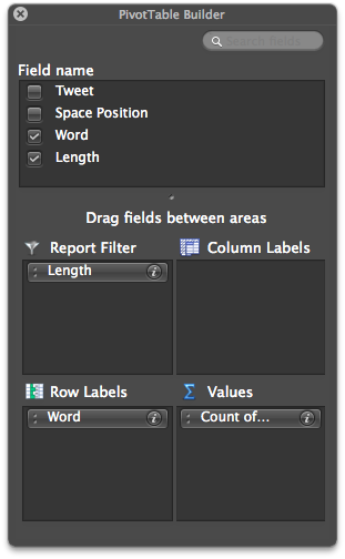
We also want to remove any words that are less than 4 characters long. We do this using the report filter drop-down menu and unchecking 0,1,2, and 3.
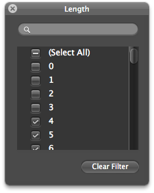
Now we need to do what is called additive smoothing: this protects your model against misrepresenting words that rarely appear – e.g. bit.ly urls are unique and so rarely appear. This is a very complicated way of saying “add 1 to everything” … in column C add 1 to all the rows in Column B and then sum them up! Your sheet should now look like this:
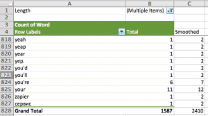
Now we can calculate the probabilities by dividing each cell in column C by the total of column C:
=C5/$C$828 |
The first thing you will notice is that the probabilities are tiny. In larger data sets they will be even tinier and perhaps Excel will not be able to handle it. So we take the natural log of the numbers using the LN() function in column D:
=LN(D5) |
Repeat all these steps for the AboutOther tab and create an Other Probability tab.
You can skip this step by downloading the file with this step completed: Mandrill – Step 4
That’s it believe it or not! You have a model.
Step 5: Using Bayes and the MAP model
So we are at a stage where we have probabilities for words in the “relevant” tweets and “irrelevant” tweets. Now what? We will now use the Maximum A Posteriori (MAP) rule that basically says, given a word if the probability of it being classified as “relevant” is higher than “irrelevant, then it’s “relevant”.
Lets demonstrate with the “TestTweets” tab. First you need to process the tweets again like we did before:
=SUBSTITUTE(B2,". "," ") =SUBSTITUTE(C2,": "," ") =SUBSTITUTE(D2,"?"," ") =SUBSTITUTE(E2,"!"," ") =SUBSTITUTE(F2,";"," ") =SUBSTITUTE(G2,","," ") |
Then create a tab called “Predictions”. In cell A1 input the label “Number” and in A2 to A21 put in the numbers 1 through 20. Label cell B2 “Prediction”. Copy and paste the values from the “TestTweets” column into C2.
Now we need to tokenize the tweets in column C. It is a lot easier this time around. All you have to do is highlight cells C2 to C21 and select “Text to Column” from the “Data” menu. You will see a pop-up screen, click next and then select “Spaces”:
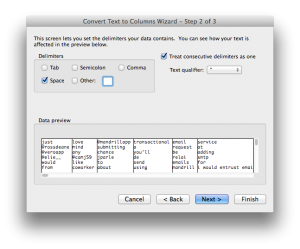
Click next and in the final screen input $D$2 as the destination cell. That’s it! All tokenized and ready for predictions … which is going to get messy 🙂
What we need to do is take each token and look up the probabilities in the “Mandrill Probability” tab and in the “Other Probability” tab. Start in cell D25 and use VLookUp() as follows:
=VLOOKUP(D2,'Mandrill Probability'!$A$5:$E$827,5,FALSE) |
Which says look up the value of D2 in the range of cells in the Mandrill Probability tab, and if you find the token, return the value in column 5 of the Mandrill Probability tab – which is the probability.
The problem here is that if you do not find the word you will have a case of a “rare word” … which we need to replace with the natural log of 1 / total smoothed tokens. So our formula will now use an if() statement and the NA() function which returns 1 or 0 if the value is found or not found respectively. We also want to throw away tokens that are shorter than 4 letters long. So we need yet another if() statement … and here is the monstrosity:
=IF(LEN(D2)<=3,0,IF(ISNA(VLOOKUP(D2,'Mandrill Probability'!$A$5:$E$827,5,FALSE)), LN(1/'Mandrill Probability'!$C$828),VLOOKUP(D2,'Mandrill Probability'!$A$5:$E$827,5,FALSE))) |
Now you can drag this down to D44 through to AI44.
Repeat this in D48 to AI for the ‘Other Probability’:
=IF(LEN(D2)<=3,0,IF(ISNA(VLOOKUP(D2,'Other Probability'!$A$5:$E$810,5,FALSE)), LN(1/'Other Probability'!$C$811),VLOOKUP(D2,'Other Probability'!$A$5:$E$810,5,FALSE))) |
Almost there, now we need to sum up each row. In cell B25 input:
=SUM(D25:AI25) |
Copy this down to B67. Now we need to compare if the top set of numbers is greater than the bottom set of numbers in our predictions. In cell B2, input the comparison:
=IF(B25>B48,"APP","OTHER") |
Drag this down to B20 to get the predictions!
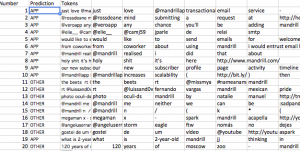
Of the 20 predicted, the model only makes a mistake on 1. That’s a pretty good margin of error.
All you need to do is repeat the steps for new tweets in the last tab. The model will deteriorate over time and therefore it is important to continuously update the model for better prediction.
You can skip this step by downloading the file with this step completed: Mandrill – Step 5
Tweet Classification with Naive Bayes Classifier: R
Step 1: Data Cleaning
We start off with our vanilla data set separated into 3 different files:
Download those files into your working directory and fire up R.
The first thing we need to do is load up the libraries we will be using and read our data. We also add the appropriate columns for “App” and “Other”:
# Libraries library(tm) # Collect data tweets.mandrill<-read.csv('Mandrill.csv',header=T) tweets.other<-read.csv('Other.csv',header=T) tweets.test<-read.csv('Test.csv',header=T) # Add "App" to mandrill tweets, and "Other" to others. tweets.mandrill["class"]<-rep("App",nrow(tweets.mandrill)) tweets.other["class"]<-rep("Other",nrow(tweets.mandrill)) |
We then need a helper function to replace all the stuff we do not want in the tweets. To do this we use a function called gsub() within our helper function.
# Helper Function replacePunctuation <- function(x) { x <- tolower(x) x <- gsub("[.]+[ ]"," ",x) x <- gsub("[:]+[ ]"," ",x) x <- gsub("[?]"," ",x) x <- gsub("[!]"," ",x) x <- gsub("[;]"," ",x) x <- gsub("[,]"," ",x) x } |
Let us do the text transformations on our tweets now:
# Do our punctuation stuff tweets.mandrill$Tweet <- replacePunctuation(tweets.mandrill$Tweet) tweets.other$Tweet <- replacePunctuation(tweets.other$Tweet) tweets.test$Tweet <- replacePunctuation(tweets.test$Tweet) |
Step 2: Word Counting
We do not need to count words for the R version. Pat yourself on the back for making a smart decision … not too much though this will get messy soon I promise 🙂

Step 3: Tokenization
We are going to use the ‘tm’ library to tokenize our training and test data. First we will create a Corpus – which is just a funky word for a set of text stuff … in this case tweets!
# Create corpus tweets.mandrill.corpus <- Corpus(VectorSource(as.vector(tweets.mandrill$Tweet))) tweets.other.corpus <- Corpus(VectorSource(as.vector(tweets.other$Tweet))) tweets.test.corpus <- Corpus(VectorSource(as.vector(tweets.test$Tweet))) |
Great! Now we want to get a term document matrix – another fancy phrase for a table that shows how many times each word was mentioned in each document.
# Create term document matrix tweets.mandrill.matrix <- t(TermDocumentMatrix(tweets.mandrill.corpus,control = list(wordLengths=c(4,Inf)))); tweets.other.matrix <- t(TermDocumentMatrix(tweets.other.corpus,control = list(wordLengths=c(4,Inf)))); tweets.test.matrix <- t(TermDocumentMatrix(tweets.test.corpus,control = list(wordLengths=c(4,Inf)))); |
This is what the term document matrix looks like:
Terms Docs which whom wisest with wordpress words 10 0 0 0 2 0 0 11 0 0 0 0 0 0 12 0 0 0 0 0 0 13 0 0 0 0 0 0 14 0 0 0 1 0 0 15 0 0 0 0 0 0 |
Great! That’s just what we need; we can count words in documents and totals later!
We can move on to building our model now.
Step 4: Model Building
We want to create the probabilities table.
- We start by counting the number of times each word has been used
- We then need to do the “additive smoothing” step
- We then take then calculate the probabilities using the smoothed frequencies
- Lastly we need to take the natural log of the probabilities
To save us time, we will write a little helper function that will do this for any document matrix we might have.
probabilityMatrix <-function(docMatrix) { # Sum up the term frequencies termSums<-cbind(colnames(as.matrix(docMatrix)),as.numeric(colSums(as.matrix(docMatrix)))) # Add one termSums<-cbind(termSums,as.numeric(termSums[,2])+1) # Calculate the probabilties termSums<-cbind(termSums,(as.numeric(termSums[,3])/sum(as.numeric(termSums[,3])))) # Calculate the natural log of the probabilities termSums<-cbind(termSums,log(as.numeric(termSums[,4]))) # Add pretty names to the columns colnames(termSums)<-c("term","count","additive","probability","lnProbability") termSums } |
Great, now we can just use that for our training sets “App” and “Other”.
tweets.mandrill.pMatrix<-probabilityMatrix(tweets.mandrill.matrix) tweets.other.pMatrix<-probabilityMatrix(tweets.other.matrix) |
We can output these to files and compare them to the Excel file:
write.csv(file="mandrillProbMatrix.csv",tweets.mandrill.pMatrix) write.csv(file="otherProbMatrix.csv",tweets.mandrill.pMatrix) |
Step 5: Using Bayes and the MAP model
We now want to use the MAP model to compare each of the test tweets with the two probability matrices.
We will write another function to help us out here. We start thinking about what we want to do with each tweet:
- Get each test tweets characters and look for them in a probability matrix
- We want to know how many words were not found.
- We want to sum up the probabilities of the found words
- For the words we do not find, we want to add ln(1/sum of the smoothed words) each time
- Sum up the probabilities from the last 2 steps
Lets go:
getProbability <- function(testChars,probabilityMatrix) { charactersFound<-probabilityMatrix[probabilityMatrix[,1] %in% testChars,"term"] # Count how many words were not found in the mandrill matrix charactersNotFound<-length(testChars)-length(charactersFound) # Add the normalized probabilities for the words founds together charactersFoundSum<-sum(as.numeric(probabilityMatrix[probabilityMatrix[,1] %in% testChars,"lnProbability"])) # We use ln(1/total smoothed words) for words not found charactersNotFoundSum<-charactersNotFound*log(1/sum(as.numeric(probabilityMatrix[,"additive"]))) #This is our probability prob<-charactersFoundSum+charactersNotFoundSum prob } |
Now we can use this function for every tweet we have with a for loop. Lets see how this is done:
# Get the matrix tweets.test.matrix<-as.matrix(tweets.test.matrix) # A holder for classification classified<-NULL for(documentNumber in 1:nrow(tweets.test.matrix)) { # Extract the test words tweets.test.chars<-names(tweets.test.matrix[documentNumber,tweets.test.matrix[documentNumber,] %in% 1]) # Get the probabilities mandrillProbability <- getProbability(tweets.test.chars,tweets.mandrill.pMatrix) otherProbability <- getProbability(tweets.test.chars,tweets.other.pMatrix) # Add it to the classification list classified<-c(classified,ifelse(mandrillProbability>otherProbability,"App","Other")) } |
Brilliant we can take a look at our classification alongside our tweets:
View(cbind(classified,tweets.test$Tweet)) |
Very much like our Excel model, we are off by 1/20.
Entire Code
library(tm) # Collect data tweets.mandrill<-read.csv('Mandrill.csv',header=T) tweets.other<-read.csv('Other.csv',header=T) tweets.test<-read.csv('Test.csv',header=T) tweets.mandrill["class"]<-rep("App",nrow(tweets.mandrill)) tweets.other["class"]<-rep("Other",nrow(tweets.mandrill)) # Helper Function replacePunctuation <- function(x) { x <- tolower(x) x <- gsub("[.]+[ ]"," ",x) x <- gsub("[:]+[ ]"," ",x) x <- gsub("[?]"," ",x) x <- gsub("[!]"," ",x) x <- gsub("[;]"," ",x) x <- gsub("[,]"," ",x) x } # Do our punctuation stuff tweets.mandrill$Tweet <- replacePunctuation(tweets.mandrill$Tweet) tweets.other$Tweet <- replacePunctuation(tweets.other$Tweet) tweets.test$Tweet <- replacePunctuation(tweets.test$Tweet) # Create corpus tweets.mandrill.corpus <- Corpus(VectorSource(as.vector(tweets.mandrill$Tweet))) tweets.other.corpus <- Corpus(VectorSource(as.vector(tweets.other$Tweet))) tweets.test.corpus <- Corpus(VectorSource(as.vector(tweets.test$Tweet))) # Create term document matrix tweets.mandrill.matrix <- t(TermDocumentMatrix(tweets.mandrill.corpus,control = list(wordLengths=c(4,Inf)))); tweets.other.matrix <- t(TermDocumentMatrix(tweets.other.corpus,control = list(wordLengths=c(4,Inf)))); tweets.test.matrix <- t(TermDocumentMatrix(tweets.test.corpus,control = list(wordLengths=c(4,Inf)))); # Probability Matrix probabilityMatrix <-function(docMatrix) { # Sum up the term frequencies termSums<-cbind(colnames(as.matrix(docMatrix)),as.numeric(colSums(as.matrix(docMatrix)))) # Add one termSums<-cbind(termSums,as.numeric(termSums[,2])+1) # Calculate the probabilties termSums<-cbind(termSums,(as.numeric(termSums[,3])/sum(as.numeric(termSums[,3])))) # Calculate the natural log of the probabilities termSums<-cbind(termSums,log(as.numeric(termSums[,4]))) # Add pretty names to the columns colnames(termSums)<-c("term","count","additive","probability","lnProbability") termSums } tweets.mandrill.pMatrix<-probabilityMatrix(tweets.mandrill.matrix) tweets.other.pMatrix<-probabilityMatrix(tweets.other.matrix) #Predict # Get the test matrix # Get words in the first document getProbability <- function(testChars,probabilityMatrix) { charactersFound<-probabilityMatrix[probabilityMatrix[,1] %in% testChars,"term"] # Count how many words were not found in the mandrill matrix charactersNotFound<-length(testChars)-length(charactersFound) # Add the normalized probabilities for the words founds together charactersFoundSum<-sum(as.numeric(probabilityMatrix[probabilityMatrix[,1] %in% testChars,"lnProbability"])) # We use ln(1/total smoothed words) for words not found charactersNotFoundSum<-charactersNotFound*log(1/sum(as.numeric(probabilityMatrix[,"additive"]))) #This is our probability prob<-charactersFoundSum+charactersNotFoundSum prob } # Get the matrix tweets.test.matrix<-as.matrix(tweets.test.matrix) # A holder for classification classified<-NULL for(documentNumber in 1:nrow(tweets.test.matrix)) { # Extract the test words tweets.test.chars<-names(tweets.test.matrix[documentNumber,tweets.test.matrix[documentNumber,] %in% 1]) # Get the probabilities mandrillProbability <- getProbability(tweets.test.chars,tweets.mandrill.pMatrix) otherProbability <- getProbability(tweets.test.chars,tweets.other.pMatrix) # Add it to the classification list classified<-c(classified,ifelse(mandrillProbability>otherProbability,"App","Other")) } View(cbind(classified,tweets.test$Tweet)) |
![]() Apr 30
Apr 30
Customer Segmentation: Excel and R
Foreward

I started reading Data Smart by John Foreman. The book is a great read because of Foreman’s humorous style of writing. What sets this book apart from the other data analysis books I have come across is that it focuses on the techniques rather than the tools – everything is accomplished through the use of a spreadsheet program (e.g. Excel).
So as a personal project to learn more about data analysis and its applications, I will be reproducing exercises in the book both in Excel and R. I will be structured in the blog posts: 0) I will always repeat this paragraph in every post 1) Introducing the Concept and Data Set, 2) Doing the Analysis with Excel, 3) Reproducing the results with R.
If you like the stuff here, please consider buying the book.
Shortcuts
This post is long, so here is a shortcut menu:
https://eternaclinic.com/skin-rejuvenation/ Excel
- Step 1: Pivot & Copy
- Step 2: Distances and Clusters
- Step 3: Solving for optimal cluster centers
- Step 4: Top deals by clusters
- Step 1: Pivot & Copy
- Step 2: Distances and Clusters
- Step 3: Solving for optimal cluster centers
- Step 4: Top deals by clusters
- Entire Code
Customer Segmentation
Customer segmentation is as simple as it sounds: grouping customers by their characteristics – and why would you want to do that? To better serve their needs!
So how does one go about segmenting customers? One method we will look at is an unsupervised method of machine learning called k-Means clustering. Unsupervised learning means finding out stuff without knowing anything about the data to start … so you want to discover.
Our example today is to do with e-mail marketing. We use the dataset from Chapter 2 on Wiley’s website – download a vanilla copy here
What we have are offers sent via email, and transactions based on those offers. What we want to do with K-Means clustering is classify customers based on offers they consume. Simplystatistics.org have a nice animation of what this might look like:
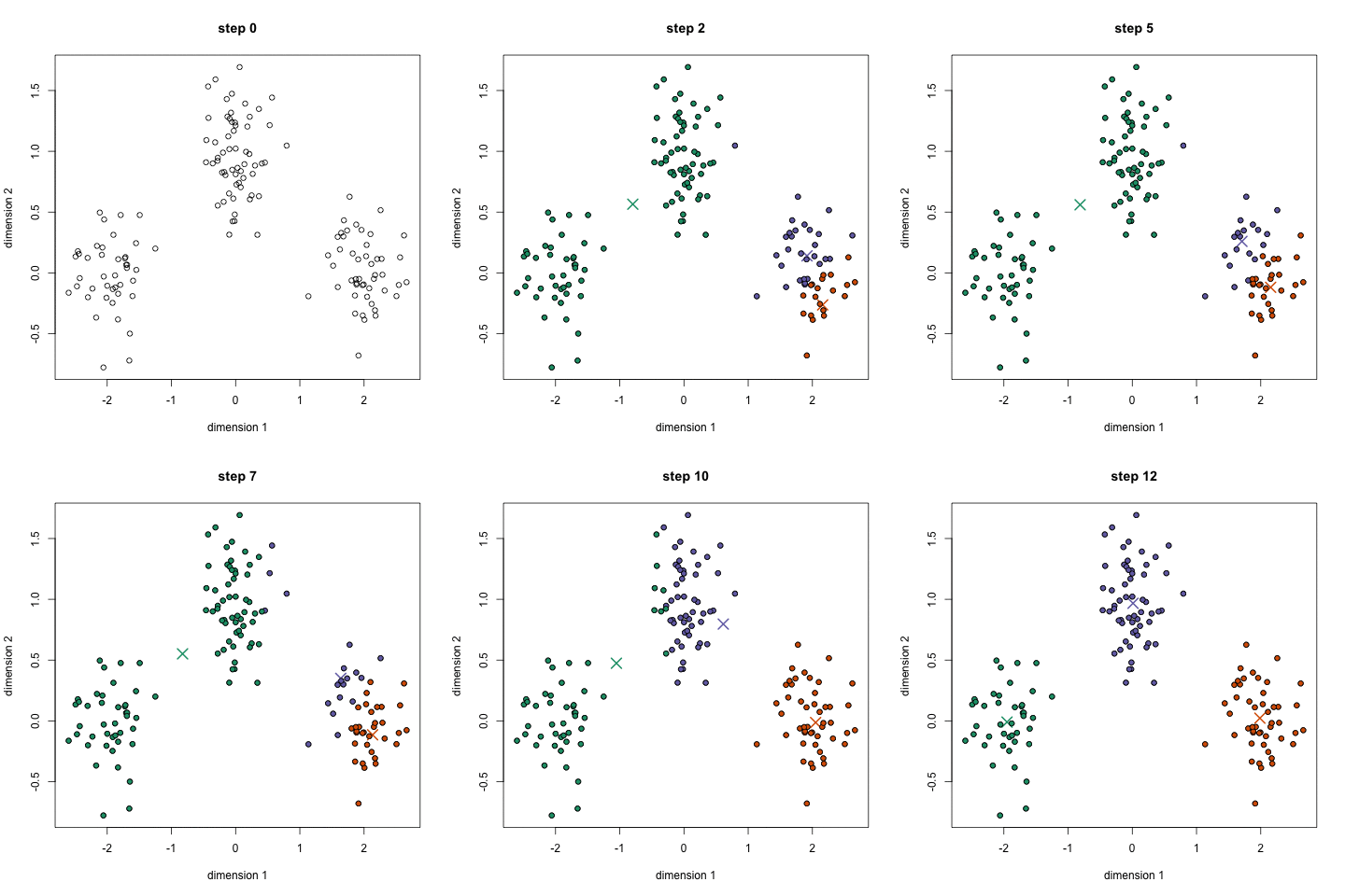
If we plot a given set of data by their dimensions, we can identify groups of similar points (customers) within the dataset by looking at how those points center around two or more points. The k in k-means is just the number of clusters you choose to identify; naturally this would be greater than one cluster.
Great, we’re ready to start.
K-Means Clustering – Excel
First what we need to do is create a transaction matrix. That means, we need to put the offers we mailed out next to the transaction history of each customer. This is easily achieved with a pivot table.
Step 1: Pivot & Copy
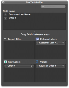 Go to your “transactions” tab and create a pivot table with the settings shown in the image to the right.
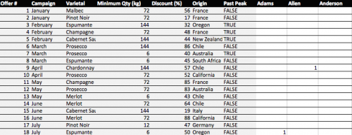
Once you have that you will have the names of the customers in columns, and the offer numbers in rows with a bunch of 1’s indicating that the customers have made a transaction based on the given offer.
Great. Copy and paste the pivot table (leaving out the grand totals column and row) into a new tab called “Matrix”.
Now copy the table from the “OfferInformation” tab and paste it to the left of your new Matrix table.
Done – You have your transaction matrix! This is what it should look like:
If you would like to skip this step, download this file with Step 1 completed.
Step 2: Distances and Clusters
We will use k = 4 indicating that we will use 4 clusters. This is somewhat arbitrary, but the number you pick should be representative of the number of segments you can handle as a business. So 100 segments does not make sense for an e-mail marketing campaign.
Lets go ahead and add 4 columns – each representing a cluster.
We need to calculate how far away each customer is from the cluster’s mean. To do this we could use many distances, one of which is the Euclidean Distance. This is basically the distance between two points using pythagorean theorem.
To do this in Excel we will use a feature called multi-cell arrays that will make our lives a lot easier. For “Adam” insert the following formula to calculate the distance from Cluster 1 and then press Ambien Buy Online CTRL+SHIFT+ENTER (if you just press enter, Excel wont know what to do):
=SQRT(SUM((L$2:L$33-$H$2:$H$33)^2)) |
Excel will automatically add braces “{}” around your formula indicating that it will run the formula for each row.
Now do the same for clusters 2, 3 and 4.
=SQRT(SUM((L$2:L$33-$I$2:$I$33)^2)) =SQRT(SUM((L$2:L$33-$J$2:$J$33)^2)) =SQRT(SUM((L$2:L$33-$K$2:$K$33)^2)) |
Now copy Adam’s 4 cells, highlight all the “distance from cluster …” cells for the rest of the customers, and paste the formula. You now have the distances for all customers.
Before moving on we need to calculate the cluster with the minimum distance. To do this we will add 2 rows: the first is “Minimum Distance” which for Adam is:
=MIN(L34:L37) |
Do the same for the remaining customers. Then add another row labelled “Assigned Cluster” with the formula:
=MATCH(L38,L34:L37,0) |
That’s all you need. Now lets go find the optimal cluster centers!
If you would like to skip this step, download this file with Step 2 completed.
Step 3: Solving for optimal cluster centers
We will use “Solver” to help us calculate the optimal centers. This step is pretty easy now that you have most of your model set up. The optimal centers will allow us to have the minimum distance for each customer – and therefore we are minimizing the total distance.
To do this, we first must know what the total distance is. So add a row under the “Assigned Cluster” and calculate the sum of the “Minimum Distance” row using the formula:
=SUM(L38:DG38) |
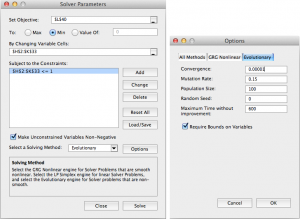
We are now ready to use solver (found in Tools -> Solver). Set up your solver to match the following screenshot.
Note that we change the solver to “evolutionary” and set options of convergence to 0.00001, and timeout to 600 seconds.
When ready, press solve. Go make yourself a coffee, this will take about 10 minutes.
Note: Foreman is able to achieve 140, I only reached 144 before my computer times out. This is largely due to my laptop’s processing power I believe. Nevertheless, the solution is largely acceptable.
I think it’s a good time to appropriately name your tab “Clusters”.
If you would like to skip this step, download this file with Step 3 completed.
Step 4: Top deals by clusters
Now we have our clusters – and essentially our segments – we want to find the top deals for each segment. That means we want to calculate, for each offer, how many were consumed by each segment.
This is easily achieved through the SUMIF function in excel. First lets set up a new tab called “Top Deals”. Copy and paste the “Offer Information” tab into your new Top Deals tab and add 4 empty columns labelled 1,2,3, and 4.
The SUMIF formula uses 3 arguments: the data you want to consider, the criteria whilst considering that data, and finally if the criteria is met what should the formula sum up. In our case we will consider the clusters as the data, the cluster number as the criteria, and the number of transactions for every offer as the final argument.
This is done using the following formula in the cell H2 (Offer 1, Cluster 1):
=SUMIF(Clusters!$L$39:$DG$39,'Top Deals'!H$1,Clusters!$L2:$DG2) |
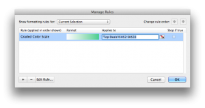
Drag this across (or copy and paste into) cells H2 to K33. You now have your top deals! It’s not very clear though so add some conditional formatting by highlighting H2:K33 and selecting format -> conditional formatting. I added the following rule:
That’s it! Foreman goes into details about how to judge whether 4 clusters are enough but this is beyond the scope of the post. We have 4 clusters and our offers assigned to each cluster. The rest is interpretation. One observation that stands out is that cluster 4 was the only cluster that consumed Offer 22.
Another is that cluster 1 have clear preferences for Pinot Noir offers and so we will push Pinot Noir offers to: Anderson, Bell, Campbell, Cook, Cox, Flores, Jenkins, Johnson, Moore, Morris, Phillips, Smith. You could even use a cosine similarity or apriori recommendations to go a step further with Cluster 1.
We are done with Excel, now lets see how to do this with R!
If you would like to skip this step, download this file with Step 4 completed.
K-Means Clustering – R
We will go through the same steps we did. We start with our vanilla files – provided in CSV format:
Download these files into a folder where you will work from in R. Fire up RStudio and lets get started.
Step 1: Pivot & Copy
First we want to read our data. This is simple enough:
# Read offers and transaction data offers<-read.csv(file="OfferInformation.csv") transactions<-read.csv(file="Transactions.csv") |
We now need to combine these 2 files to get a frequency matrix – equivalent to pivoting in Excel. This can be done using the reshape library in R. Specifically we will use the melt and cast functions.
We first melt the 2 columns of the transaction data. This will create data that we can pivot: customer, variable, and value. We only have 1 variable here – Offer.
We then want to cast this data by putting value first (the offer number) in rows, customer names in the columns. This is done by using R’s style of formula input: Value ~ Customers.
We then want to count each occurrence of customers in the row. This can be done by using a function that takes customer names as input, counts how many there are, and returns the result. Simply: function(x) length(x)
Lastly, we want to combine the data from offers with our new transaction matrix. This is done using cbind (column bind) which glues stuff together automagically.
Lots of explanations for 3 lines of code!
#Load Library library(reshape) # Melt transactions, cast offer by customers pivot<-melt(transactions[1:2]) pivot<-(cast(pivot,value~Customer.Last.Name,fill=0,fun.aggregate=function(x) length(x))) # Bind to offers, we remove the first column of our new pivot because it's redundant. pivot<-cbind(offers,pivot[-1]) |
We can output the pivot table into a new CSV file called pivot.
write.csv(file="pivot.csv",pivot)
Step 2: Clustering
To cluster the data we will use only the columns starting from “Adams” until “Young”.
We will use the fpc library to run the KMeans algorithm with 4 clusters.
To use the algorithm we will need to rotate the transaction matrix with t().
That’s all you need: 4 lines of code!
# Load library library(fpc) # Only use customer transaction data and we will rotate the matrix cluster.data<-pivot[,8:length(pivot)] cluster.data<-t(cluster.data) # We will run KMeans using pamk (more robust) with 4 clusters. cluster.kmeans<-pamk(cluster.data,k=4) # Use this to view the clusters View(cluster.kmeans$pamobject$clustering) |
Step 3: Solving for Cluster Centers
This is not a necessary step in R! Pat yourself on the back, get another cup of tea or coffee and move onto to step 4.
Step 4: Top deals by clusters
Top get the top deals we will have to do a little bit of data manipulation. First we need to combine our clusters and transactions. Noteably the lengths of the ‘tables’ holding transactions and clusters are different. So we need a way to merge the data … so we use the merge() function and give our columns sensible names:
#Merge Data cluster.deals<-merge(transactions[1:2],cluster.kmeans$pamobject$clustering,by.x = "Customer.Last.Name", by.y = "row.names") colnames(cluster.deals)<-c("Name","Offer","Cluster") |
We then want to repeat the pivoting process to get Offers in rows and clusters in columns counting the total number of transactions for each cluster. Once we have our pivot table we will merge it with the offers data table like we did before:
# Melt, cast, and bind cluster.pivot<-melt(cluster.deals,id=c("Offer","Cluster")) cluster.pivot<-cast(cluster.pivot,Offer~Cluster,fun.aggregate=length) cluster.topDeals<-cbind(offers,cluster.pivot[-1]) |
We can then reproduce the excel version by writing to a csv file:
write.csv(file="topdeals.csv",cluster.topDeals,row.names=F) |
Note
It’s important to note that cluster 1 in excel does not correspond to cluster 1 in R. It’s just the way the algorithms run. Moreover, the allocation of clusters might differ slightly because of the nature of kmeans algorithm. However, your insights will be the same; in R we also see that cluster 3 prefers Pinot Noir and cluster 4 has a strong preference for Offer 22.
Entire Code
# Read data offers<-read.csv(file="OfferInformation.csv") transactions<-read.csv(file="Transactions.csv") # Create transaction matrix library(reshape) pivot<-melt(transactions[1:2]) pivot<-(cast(pivot,value~Customer.Last.Name,fill=0,fun.aggregate=function(x) length(x))) pivot<-cbind(offers,pivot[-1]) write.csv(file="pivot.csv",pivot) # Cluster library(fpc) cluster.data<-pivot[,8:length(pivot)] cluster.data<-t(cluster.data) cluster.kmeans<-pamk(cluster.data,k=4) # Merge Data cluster.deals<-merge(transactions[1:2],cluster.kmeans$pamobject$clustering,by.x = "Customer.Last.Name", by.y = "row.names") colnames(cluster.deals)<-c("Name","Offer","Cluster") # Get top deals by cluster cluster.pivot<-melt(cluster.deals,id=c("Offer","Cluster")) cluster.pivot<-cast(cluster.pivot,Offer~Cluster,fun.aggregate=length) cluster.topDeals<-cbind(offers,cluster.pivot[-1]) write.csv(file="topdeals.csv",cluster.topDeals,row.names=F) |
![]() Apr 26
Apr 26
Collaborative Filtering with R
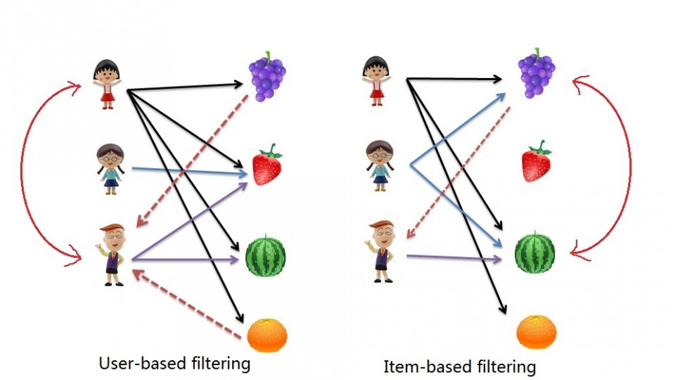
We already looked at Market Basket Analysis with R. https://www.leoosborne.com/bronze-sculptures/ Collaborative filtering is another technique that can be used for recommendation.
The underlying concept behind this technique is as follows:
- Assume Person A likes Oranges, and Person B likes Oranges.
- Assume Person A likes Apples.
- Person B is likely to have similar opinions on Apples as A than some other random person.
The implications of collaborative filtering are obvious: you can predict and recommend items to users based on preference similarities. There are two types of collaborative filtering: user-based and item-based.
follow url Item Based Collaborative Filtering takes the similarities between items’ consumption history.
https://www.aminhaclinica.com.br/consultas/ User Based Collaborative Filtering considers similarities between user consumption history.
We will look at both types of collaborative filtering using a publicly available dataset from LastFM.
Case: Last.FM Music
The data set contains information about users, their gender, their age, and which artists they have listened to on Last.FM. We will not use the entire dataset. For simplicity’s sake we only use songs in Germany and we will transform the data to a item frequency matrix. This means each row will represent a user, and each column represents and artist. For this we use R’s “reshape” package. This is largely administrative, so we will start with the transformed dataset.
Download the LastFM Germany frequency matrix and put it in your working directory. Load up R and read the data file.
# Read data from Last.FM frequency matrix data.germany <- read.csv(file="lastfm-matrix-germany.csv") |
Lets look at a sample of our data. The output looks something like this:
head(data.germany[,c(1,3:8)]) user abba ac.dc adam.green aerosmith afi air 1 1 0 0 0 0 0 0 2 33 0 0 1 0 0 0 3 42 0 0 0 0 0 0 4 51 0 0 0 0 0 0 5 62 0 0 0 0 0 0 6 75 0 0 0 0 0 0 |
We’re good to go!
Item Based Collaborative Filtering
In item based collaborative filtering we do not really care about the users. So the first thing we should do is drop the user column from our data. This is really easy since it is the first column, but if it was not the first column we would still be able to drop it with the following code:
# Drop any column named "user" data.germany.ibs <- (data.germany[,!(names(data.germany) %in% c("user"))]) |
We then want to calculate the similarity of each song with the rest of the songs. This means that we want to compare each column in our “data.germany.ibs” data set with every other column in the data set. Specifically, we will be comparing what is known as the “Cosine Similarity”.
The cosine similarity, in essence takes the sum product of the first and second column, and divide that by the product of the square root of the sum of squares of each column. (that was a mouth-full!)
The important thing to know is the resulting number represents how “similar” the first column is with the second column. We will use the following helper function to product the Cosine Similarity:
# Create a helper function to calculate the cosine between two vectors getCosine <- function(x,y) { this.cosine <- sum(x*y) / (sqrt(sum(x*x)) * sqrt(sum(y*y))) return(this.cosine) } |
We are now ready to start comparing each of our songs (items). We first need a placeholder to store the results of our cosine similarities. This placeholder will have the songs in both columns and rows:
# Create a placeholder dataframe listing item vs. item data.germany.ibs.similarity <- matrix(NA, nrow=ncol(data.germany.ibs),ncol=ncol(data.germany.ibs),dimnames=list(colnames(data.germany.ibs),colnames(data.germany.ibs))) |
The first 6 items of the empty placeholder will look like this:
a.perfect.circle abba ac.dc adam.green aerosmith afi a.perfect.circle NA NA NA NA NA NA abba NA NA NA NA NA NA ac.dc NA NA NA NA NA NA adam.green NA NA NA NA NA NA aerosmith NA NA NA NA NA NA afi NA NA NA NA NA NA |
Perfect, all that’s left is to loop column by column and calculate the cosine similarities with our helper function, and then put the results into the placeholder data table. That sounds like a pretty straight-forward nested for-loop:
# Lets fill in those empty spaces with cosine similarities # Loop through the columns for(i in 1:ncol(data.germany.ibs)) { # Loop through the columns for each column for(j in 1:ncol(data.germany.ibs)) { # Fill in placeholder with cosine similarities data.germany.ibs.similarity[i,j] <- getCosine(as.matrix(data.germany.ibs[i]),as.matrix(data.germany.ibs[j])) } } # Back to dataframe data.germany.ibs.similarity <- as.data.frame(data.germany.ibs.similarity) |
Note: For loops in R are infernally slow. We use as.matrix() to transform the columns into matrices since matrix operations run a lot faster. We transform the similarity matrix into a data.frame for later processes that we will use.
We have our similarity matrix. Now the question is … Xanax Buy Without Prescription so what?
We are now in a position to make recommendations! We look at the top 10 neighbours of each song – those would be the recommendations we make to people listening to those songs.
We start off by creating a placeholder:
# Get the top 10 neighbours for each data.germany.neighbours <- matrix(NA, nrow=ncol(data.germany.ibs.similarity),ncol=11,dimnames=list(colnames(data.germany.ibs.similarity))) |
Our empty placeholder should look like this:
[,1] [,2] [,3] [,4] [,5] [,6] [,7] [,8] [,9] [,10] [,11] a.perfect.circle NA NA NA NA NA NA NA NA NA NA NA abba NA NA NA NA NA NA NA NA NA NA NA ac.dc NA NA NA NA NA NA NA NA NA NA NA adam.green NA NA NA NA NA NA NA NA NA NA NA aerosmith NA NA NA NA NA NA NA NA NA NA NA afi NA NA NA NA NA NA NA NA NA NA NA |
Then we need to find the neighbours. This is another loop but runs much faster.
for(i in 1:ncol(data.germany.ibs)) { data.germany.neighbours[i,] <- (t(head(n=11,rownames(data.germany.ibs.similarity[order(data.germany.ibs.similarity[,i],decreasing=TRUE),][i])))) } |
It’s a little bit more complicated so lets break it down into steps:
- We loop through all our artists
- We sort our similarity matrix for the artist so that we have the most similar first.
- We take the top 11 (first will always be the same artist) and put them into our placeholder
- Note we use t() to rotate the similarity matrix since the neighbour one is shaped differently
The filled in placeholder should look like this:
[,1] [,2] [,3] a.perfect.circle "a.perfect.circle" "tool" "dredg" abba "abba" "madonna" "robbie.williams" ac.dc "ac.dc" "red.hot.chilli.peppers" "metallica" adam.green "adam.green" "the.libertines" "the.strokes" aerosmith "aerosmith" "u2" "led.zeppelin" afi "afi" "funeral.for.a.friend" "rise.against" |
This means for those listening to Abba we would recommend Madonna and Robbie Williams.
Likewise for people listening to ACDC we would recommend the Red Hot Chilli Peppers and Metallica.
User Based Recommendations
We will need our similarity matrix for User Based recommendations.
The process behind creating a score matrix for the User Based recommendations is pretty straight forward:
- Choose an item and check if a user consumed that item
- Get the similarities of that item’s top X neighbours
- Get the consumption record of the user of the top X neighbours
- Calculate the score with a formula: sumproduct(purchaseHistory, similarities)/sum(similarities)
We can start by creating a helper function to calculate the score mentioned in the last step.
# Lets make a helper function to calculate the scores getScore <- function(history, similarities) { x <- sum(history*similarities)/sum(similarities) x } |
We will also need a holder matrix. We will use the original data set now (data.germany):
# A placeholder matrix holder <- matrix(NA, nrow=nrow(data.germany),ncol=ncol(data.germany)-1,dimnames=list((data.germany$user),colnames(data.germany[-1]))) |
The rest is one big ugly nested loop. First the loop, then we will break it down step by step:
# Loop through the users (rows) for(i in 1:nrow(holder)) { # Loops through the products (columns) for(j in 1:ncol(holder)) { # Get the user's name and th product's name # We do this not to conform with vectors sorted differently user <- rownames(holder)[i] product <- colnames(holder)[j] # We do not want to recommend products you have already consumed # If you have already consumed it, we store an empty string if(as.integer(data.germany[data.germany$user==user,product]) == 1) { holder[i,j]<-"" } else { # We first have to get a product's top 10 neighbours sorted by similarity topN<-((head(n=11,(data.germany.ibs.similarity[order(data.germany.ibs.similarity[,product],decreasing=TRUE),][product])))) topN.names <- as.character(rownames(topN)) topN.similarities <- as.numeric(topN[,1]) # Drop the first one because it will always be the same song topN.similarities<-topN.similarities[-1] topN.names<-topN.names[-1] # We then get the user's purchase history for those 10 items topN.purchases<- data.germany[,c("user",topN.names)] topN.userPurchases<-topN.purchases[topN.purchases$user==user,] topN.userPurchases <- as.numeric(topN.userPurchases[!(names(topN.userPurchases) %in% c("user"))]) # We then calculate the score for that product and that user holder[i,j]<-getScore(similarities=topN.similarities,history=topN.userPurchases) } # close else statement } # end product for loop } # end user for loop data.germany.user.scores <- holder |
The loop starts by taking each user (row) and then jumps into another loop that takes each column (artists).
We then store the user’s name and artist name in variables to use them easily later.
We then use an if statement to filter out artists that a user has already listened to – this is a business case decision.
The next bit gets the item based similarity scores for the artist under consideration.
# We first have to get a product's top 10 neighbours sorted by similarity topN<-((head(n=11,(data.germany.ibs.similarity[order(data.germany.ibs.similarity[,product],decreasing=TRUE),][product])))) topN.names <- as.character(rownames(topN)) topN.similarities <- as.numeric(topN[,1]) # Drop the first one because it will always be the same song topN.similarities<-topN.similarities[-1] topN.names<-topN.names[-1] |
It is important to note the number of artists you pick matters. We pick the top 10.
We store the similarities score and song names.
We also drop the first column because, as we saw, it always represents the same song.
We’re almost there. We just need the user’s purchase history for the top 10 songs.
# We then get the user's purchase history for those 10 items topN.purchases<- data.germany[,c("user",topN.names)] topN.userPurchases<-topN.purchases[topN.purchases$user==user,] topN.userPurchases <- as.numeric(topN.userPurchases[!(names(topN.userPurchases) %in% c("user"))]) |
We use the original data set to get the purchases of our users’ top 10 purchases.
We filter out our current user in the loop and then filter out purchases that match the user.
We are now ready to calculate the score and store it in our holder matrix:
# We then calculate the score for that product and that user holder[i,j]<-getScore(similarities=topN.similarities,history=topN.userPurchases) |
Once we are done we can store the results in a data frame.
The results should look something like this:
X a.perfect.circle abba ac.dc 1 0.0000000 0.00000000 0.20440540 33 0.0823426 0.00000000 0.09591153 42 0.0000000 0.08976655 0.00000000 51 0.0823426 0.08356811 0.00000000 62 0.0000000 0.00000000 0.11430459 75 0.0000000 0.00000000 0.00000000 |
This basically reads that for user 51 we would recommend abba first, then a perfect circle, and we would not recommend ACDC.
This is not very pretty … so lets make it pretty:
We will create another holder matrix and for each user score we will sort the scores and store the artist names in rank order.
# Lets make our recommendations pretty data.germany.user.scores.holder <- matrix(NA, nrow=nrow(data.germany.user.scores),ncol=100,dimnames=list(rownames(data.germany.user.scores))) for(i in 1:nrow(data.germany.user.scores)) { data.germany.user.scores.holder[i,] <- names(head(n=100,(data.germany.user.scores[,order(data.germany.user.scores[i,],decreasing=TRUE)])[i,])) } |
The output of this will look like this:
X V1 V2 V3 1 flogging.molly coldplay aerosmith 33 peter.fox gentleman red.hot.chili.peppers 42 oomph. lacuna.coil rammstein 51 the.subways the.kooks the.hives 62 mando.diao the.fratellis jack.johnson 75 hoobastank papa.roach the.prodigy |
By sorting we see that actually the top 3 for user 51 is the subways, the kooks, and the hives!
References
- Data Mining and Business Analytics with R
- This case is based on Professor Miguel Canela “Designing a music recommendation app”
Entire Code
# Admin stuff here, nothing special options(digits=4) data <- read.csv(file="lastfm-data.csv") data.germany <- read.csv(file="lastfm-matrix-germany.csv") ############################ # Item Based Similarity # ############################ # Drop the user column and make a new data frame data.germany.ibs <- (data.germany[,!(names(data.germany) %in% c("user"))]) # Create a helper function to calculate the cosine between two vectors getCosine <- function(x,y) { this.cosine <- sum(x*y) / (sqrt(sum(x*x)) * sqrt(sum(y*y))) return(this.cosine) } # Create a placeholder dataframe listing item vs. item holder <- matrix(NA, nrow=ncol(data.germany.ibs),ncol=ncol(data.germany.ibs),dimnames=list(colnames(data.germany.ibs),colnames(data.germany.ibs))) data.germany.ibs.similarity <- as.data.frame(holder) # Lets fill in those empty spaces with cosine similarities for(i in 1:ncol(data.germany.ibs)) { for(j in 1:ncol(data.germany.ibs)) { data.germany.ibs.similarity[i,j]= getCosine(data.germany.ibs[i],data.germany.ibs[j]) } } # Output similarity results to a file write.csv(data.germany.ibs.similarity,file="final-germany-similarity.csv") # Get the top 10 neighbours for each data.germany.neighbours <- matrix(NA, nrow=ncol(data.germany.ibs.similarity),ncol=11,dimnames=list(colnames(data.germany.ibs.similarity))) for(i in 1:ncol(data.germany.ibs)) { data.germany.neighbours[i,] <- (t(head(n=11,rownames(data.germany.ibs.similarity[order(data.germany.ibs.similarity[,i],decreasing=TRUE),][i])))) } # Output neighbour results to a file write.csv(file="final-germany-item-neighbours.csv",x=data.germany.neighbours[,-1]) ############################ # User Scores Matrix # ############################ # Process: # Choose a product, see if the user purchased a product # Get the similarities of that product's top 10 neighbours # Get the purchase record of that user of the top 10 neighbours # Do the formula: sumproduct(purchaseHistory, similarities)/sum(similarities) # Lets make a helper function to calculate the scores getScore <- function(history, similarities) { x <- sum(history*similarities)/sum(similarities) x } # A placeholder matrix holder <- matrix(NA, nrow=nrow(data.germany),ncol=ncol(data.germany)-1,dimnames=list((data.germany$user),colnames(data.germany[-1]))) # Loop through the users (rows) for(i in 1:nrow(holder)) { # Loops through the products (columns) for(j in 1:ncol(holder)) { # Get the user's name and th product's name # We do this not to conform with vectors sorted differently user <- rownames(holder)[i] product <- colnames(holder)[j] # We do not want to recommend products you have already consumed # If you have already consumed it, we store an empty string if(as.integer(data.germany[data.germany$user==user,product]) == 1) { holder[i,j]<-"" } else { # We first have to get a product's top 10 neighbours sorted by similarity topN<-((head(n=11,(data.germany.ibs.similarity[order(data.germany.ibs.similarity[,product],decreasing=TRUE),][product])))) topN.names <- as.character(rownames(topN)) topN.similarities <- as.numeric(topN[,1]) # Drop the first one because it will always be the same song topN.similarities<-topN.similarities[-1] topN.names<-topN.names[-1] # We then get the user's purchase history for those 10 items topN.purchases<- data.germany[,c("user",topN.names)] topN.userPurchases<-topN.purchases[topN.purchases$user==user,] topN.userPurchases <- as.numeric(topN.userPurchases[!(names(topN.userPurchases) %in% c("user"))]) # We then calculate the score for that product and that user holder[i,j]<-getScore(similarities=topN.similarities,history=topN.userPurchases) } # close else statement } # end product for loop } # end user for loop # Output the results to a file data.germany.user.scores <- holder write.csv(file="final-user-scores.csv",data.germany.user.scores) # Lets make our recommendations pretty data.germany.user.scores.holder <- matrix(NA, nrow=nrow(data.germany.user.scores),ncol=100,dimnames=list(rownames(data.germany.user.scores))) for(i in 1:nrow(data.germany.user.scores)) { data.germany.user.scores.holder[i,] <- names(head(n=100,(data.germany.user.scores[,order(data.germany.user.scores[i,],decreasing=TRUE)])[i,])) } # Write output to file write.csv(file="final-user-recommendations.csv",data.germany.user.scores.holder) |
![]() Apr 7
Apr 7
Kuwait Stock Exchange P/E with R

Foreword
I was inspired by Meet Saptarsi’s post on R-Bloggers.com and decided to emulate the process for the Kuwait Stock Exchange.
go Disclaimer This is not financial advice of any sort! I did this to demonstrate how R can be used to scrape information about the Kuwait Stock Exchange listed companies and do basic data analysis on the data.
Dig in!
First we want to set up the libraries we will use in our script.
We will be using XML to scrape websites and GGPlot2 to create our graphs.
library(XML) library('ggplot2') |
Kuwait Stock Exchange – Ticker Symbols
Initially I thought we could get all the information we want from the Kuwait stock exchange (KSE) website. I was terribly mistaken. KSE.com.kw is so behind the times … but atleast we can accurately gather the ticker names of companies listed in the KSE.
The process is simple.
- Find the page with information you want: http://www.kuwaitse.com/Stock/Companies.aspx
- Use readHTMLTable() to read the page, and find a table. In this case it’s table #35
- Now you have a data frame that you can access the tickers!
# Read Stock Information from KSE kse.url <- "http://www.kuwaitse.com/Stock/Companies.aspx" tables <- readHTMLTable(kse.url,head=T,which=35) tickers<-tables$Ticker |
P/E Ratios
P/E ratios are used to guage growth expectations of a company compared to others within a sector. You can find details about the P/E ratio here, but we will suffice by saying that we want to know what the market looks like in terms of P/E ratios.
Ideally the P/E ratio would be available from KSE or atleast access to digital forms of each company's financial statements. I was unable to find such a thing so I turned to MarketWatch.com. We can use the ticker codes we collected to grab the data we need.
The process is different because MarketWatch does not have HTML tables. Instead the process is slightly more complicated.
- Create a holder data frame
- Loop through each ticker and point to the relevant page:
http://www.marketwatch.com/investing/Stock/ https://tuf-top.com/about-us/ TICKER-NAME?countrycode=KW
Replacing TICKER-NAME with the ticker name - We go through the HTML elements of the page until we find the P/E Ratio
- Once we have collected all the P/E ratios, we do some data cleaning and we’re done!
What’s interesting is that after the data cleansing we lose 40 odd companies because there is no data available on their P/E ratios. This could also mean that these companies are losing money … because companies with no earnings have no P/E ratio! Realistically this is not a large number to hunt for but we omit them for the sake of simplicity here.
# Create an empty frame first pe.data <- data.frame('Ticker'='','PE'='') pe.data <- pe.data[-1,] # Loop through the ticker symbols for(i in 1:length(tickers)) { this.ticker<-tickers[i] # Set up the URL to use this.url <- paste("http://www.marketwatch.com/investing/Stock/",tickers[i],"?countrycode=KW",sep="") # Get the page source this.doc <- htmlTreeParse(this.url, useInternalNodes = T) # We can look at the HTML parts that contain the PE ratio this.nodes<-getNodeSet(this.doc, "//div[@class='section']//p") # We look for the value of the PE ratio within the nodes this.pe<-suppressWarnings(as.numeric(sapply(this.nodes[4], xmlValue,'data'))) # Add a row to the P/E data frame and move onto the next ticker! symbol pe.data<-rbind(pe.data,data.frame('Ticker'=this.ticker,'PE'=this.pe)) } # Combine the P/E data frame with the KSE ticker data frame combined<-(cbind(tables,pe.data)) # Lets do some data cleaning removing the 'NAs' combined.clean<-(combined[!(combined$PE %in% NA),]) # We attach our data frame to use the names of columns as variables attach(combined.clean) |
Data Exploration
We draw a box plot and output summary statistics.
We see that we have a number of outliers and generally the majority of P/E ratios are centered around 20.94.
boxplot(PE,col='blue') summary(PE) |
## Min. 1st Qu. Median Mean 3rd Qu. Max. ## 1.93 9.55 13.00 20.90 20.80 240.00 |
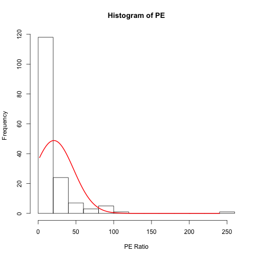
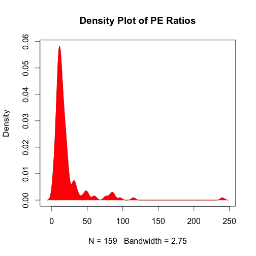
To see the spread we can look at a histogram or a density plot.
Both plots confirm a strong skew in the PE ratios.
# We can make a histogram histogram<-hist(PE,xlab="PE Ratio") # Draw a normal curve xfit<-seq(min(PE),max(PE)) yfit<-dnorm(xfit,mean=mean(PE),sd=sd(PE)) yfit <- yfit*diff(histogram$mids[1:2])*length(PE) lines(xfit, yfit, col="red", lwd=2) |
# Alternatively we can use a density plot plot(density(PE),main="Density Play of PE Ratios") polygon(density(PE), col="red", border="red",lwd=1) |
Scatter plot by industry
Lets get with it then.
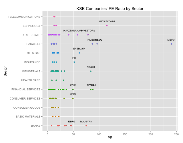
We want to see a plot of the P/E ratios by industry.
# We will want to highlihgt the outliers so lets get the outliers from our box plot outliers<-combined.clean[(which(PE %in% (boxplot.stats(PE)$out))),] # Lets create a Scatter Plot highlighting our outliers qplot(PE,Sector,main="KSE Companies' PE Ratio by Sector") + geom_point(aes(colour=Sector)) + geom_text(data=outliers,aes(label=outliers$Ticker),vjust=-2,cex=3)+ theme(legend.position = "none") |
We can clearly see the outliers. Generally outliers should tell you that something is fundamentally wrong. A company with a super high P/E ratio compared to its peers means that they have had terrible earnings, that investor expect some sort of extraordinary performance irrespective of the price, or that there is something fundamentally questionable about the numbers and you should dig in deeper. For details you can check out Investopedia.com
# Lets print out the outlier names (data.frame(outliers$Sector,outliers$Name)) |
## outliers.Sector outliers.Name ## 1 OIL & GAS THE ENERGY HOUSE CO ## 2 INDUSTRIALS NATIONAL INDUSTRIES COMPANY ## 3 CONSUMER SERVICES UNITED FOODSTUFF INDUSTRIES GROUP CO. ## 4 BANKS COMMERCIAL BANK OF KUWAIT ## 5 BANKS BURGAN BANK ## 6 BANKS BOUBYAN BANK ## 7 INSURANCE FIRST TAKAFUL INSURANCE COMPANY ## 8 REAL ESTATE INJAZZAT REAL ESTATE DEV. CO ## 9 REAL ESTATE INVESTORS HOLDING GROUP CO. ## 10 REAL ESTATE SANAM REAL ESTATE CO. ## 11 FINANCIAL SERVICES FIRST INVESTMENT COMPANY ## 12 FINANCIAL SERVICES OSOUL INVESTMENT CO. ## 13 FINANCIAL SERVICES KUWAIT CHINA INVESTMENT COMPANY ## 14 TECHNOLOGY HAYAT COMMUNICATIONS COMPANY ## 15 PARALLEL AL-BAREEQ HOLDING CO. ## 16 PARALLEL AL-MAIDAN CLINIC FOR ORAL HEALTH SERVICES CO. ## 17 PARALLEL DAR AL THURAYA REAL ESTATE CO. |
![]() Mar 19
Mar 19
Market Basket Analysis with R
Association Rules
There are many ways to see the similarities between items. These are techniques that fall under the general umbrella of source url association. The outcome of this type of technique, in simple terms, is a set of rules that can be understood as Order Clonazepam Online “if this, then that”.
Applications
So what kind of items are we talking about?
There are many applications of association:
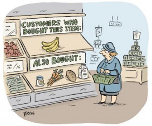
- Product recommendation – like Amazon’s “customers who bought that, also bought this”
- Music recommendations – like Last FM’s artist recommendations
- Medical diagnosis – like with diabetes really cool stuff
- Content optimisation – like in magazine websites or blogs
In this post we will focus on the retail application – it is simple, intuitive, and the dataset comes packaged with R making it repeatable.
The Groceries Dataset
Imagine 10000 receipts sitting on your table. Each receipt represents a transaction with items that were purchased. The receipt is a representation of stuff that went into a customer’s basket – and therefore ‘Market Basket Analysis’.
That is exactly what the Groceries Data Set contains: a collection of receipts with each line representing 1 receipt and the items purchased. Each line is called a source transaction and each column in a row represents an Purchase Ambien Online item. You can download the Groceries data set to take a look at it, but this is not a necessary step.
A little bit of Math
We already discussed the concept of Items and Item Sets.
We can represent our items as an item set as follows:
Therefore a transaction is represented as follows:
This gives us our rules which are represented as follows:
Which can be read as “if a user buys an item in the item set on the left hand side, then the user will likely buy the item on the right hand side too”. A more human readable example is:
If a customer buys coffee and sugar, then they are also likely to buy milk.
With this we can understand three important ratios; the support, confidence and lift. We describe the significance of these in the following bullet points, but if you are interested in a formal mathematical definition you can find it on wikipedia.
- Support: The fraction of which our item set occurs in our dataset.
- Confidence: probability that a rule is correct for a new transaction with items on the left.
- Lift: The ratio by which by the confidence of a rule exceeds the expected confidence.
Note: if the lift is 1 it indicates that the items on the left and right are independent. - We set the minimum support to 0.001
- We set the minimum confidence of 0.8
- We then show the top 5 rules
- The number of rules generated: 410
- The distribution of rules by length: Most rules are 4 items long
- The summary of quality measures: interesting to see ranges of support, lift, and confidence.
- The information on the data mined: total data mined, and minimum parameters.
- What are customers likely to buy before buying whole milk
- What are customers likely to buy if they purchase whole milk?
- We set the confidence to 0.15 since we get no rules with 0.8
- We set a minimum length of 2 to avoid empty left hand side items
- Snowplow Market Basket Analysis
- Discovering Knowledge in Data: An Introduction to Data Mining
- RDatamining.com
Apriori Recommendation with R
So lets get started by loading up our libraries and data set.
# Load the libraries library(arules) library(arulesViz) library(datasets) # Load the data set data(Groceries) |
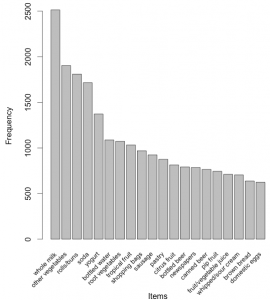
Lets explore the data before we make any rules:
# Create an item frequency plot for the top 20 items itemFrequencyPlot(Groceries,topN=20,type="absolute") |
We are now ready to mine some rules!
You will always have to pass the minimum required support and confidence.
# Get the rules rules <- apriori(Groceries, parameter = list(supp = 0.001, conf = 0.8)) # Show the top 5 rules, but only 2 digits options(digits=2) inspect(rules[1:5]) |
The output we see should look something like this
lhs rhs support confidence lift 1 {liquor,red/blush wine} => {bottled beer} 0.0019 0.90 11.2 2 {curd,cereals} => {whole milk} 0.0010 0.91 3.6 3 {yogurt,cereals} => {whole milk} 0.0017 0.81 3.2 4 {butter,jam} => {whole milk} 0.0010 0.83 3.3 5 {soups,bottled beer} => {whole milk} 0.0011 0.92 3.6 |
This reads easily, for example: if someone buys yogurt and cereals, they are 81% likely to buy whole milk too.
We can get summary info. about the rules that give us some interesting information such as:
set of 410 rules rule length distribution (lhs + rhs): sizes 3 4 5 6 29 229 140 12 summary of quality measures: support conf. lift Min. :0.00102 Min. :0.80 Min. : 3.1 1st Qu.:0.00102 1st Qu.:0.83 1st Qu.: 3.3 Median :0.00122 Median :0.85 Median : 3.6 Mean :0.00125 Mean :0.87 Mean : 4.0 3rd Qu.:0.00132 3rd Qu.:0.91 3rd Qu.: 4.3 Max. :0.00315 Max. :1.00 Max. :11.2 mining info: data n support confidence Groceries 9835 0.001 0.8 |
Sorting stuff out
The first issue we see here is that the rules are not sorted. Often we will want the most relevant rules first. Lets say we wanted to have the most likely rules. We can easily sort by confidence by executing the following code.
rules<-sort(rules, by="confidence", decreasing=TRUE) |
Now our top 5 output will be sorted by confidence and therefore the most relevant rules appear.
lhs rhs support conf. lift 1 {rice,sugar} => {whole milk} 0.0012 1 3.9 2 {canned fish,hygiene articles} => {whole milk} 0.0011 1 3.9 3 {root vegetables,butter,rice} => {whole milk} 0.0010 1 3.9 4 {root vegetables,whipped/sour cream,flour} => {whole milk} 0.0017 1 3.9 5 {butter,soft cheese,domestic eggs} => {whole milk} 0.0010 1 3.9 |
Rule 4 is perhaps excessively long. Lets say you wanted more concise rules. That is also easy to do by adding a “maxlen” parameter to your apriori function:
rules <- apriori(Groceries, parameter = list(supp = 0.001, conf = 0.8,maxlen=3)) |
Redundancies
Sometimes, rules will repeat. Redundancy indicates that one item might be a given. As an analyst you can elect to drop the item from the dataset. Alternatively, you can remove redundant rules generated.
We can eliminate these repeated rules using the follow snippet of code:
subset.matrix <- is.subset(rules, rules) subset.matrix[lower.tri(subset.matrix, diag=T)] <- NA redundant <- colSums(subset.matrix, na.rm=T) >= 1 rules.pruned <- rules[!redundant] rules<-rules.pruned |
Targeting Items
Now that we know how to generate rules, limit the output, lets say we wanted to target items to generate rules. There are two types of targets we might be interested in that are illustrated with an example of “whole milk”:
This essentially means we want to set either the Left Hand Side and Right Hand Side. This is not difficult to do with R!
Answering the first question we adjust our apriori() function as follows:
rules<-apriori(data=Groceries, parameter=list(supp=0.001,conf = 0.08), appearance = list(default="lhs",rhs="whole milk"), control = list(verbose=F)) rules<-sort(rules, decreasing=TRUE,by="confidence") inspect(rules[1:5]) |
The output will look like this:
lhs rhs supp. conf. lift 1 {rice,sugar} => {whole milk} 0.0012 1 3.9 2 {canned fish,hygiene articles} => {whole milk} 0.0011 1 3.9 3 {root vegetables,butter,rice} => {whole milk} 0.0010 1 3.9 4 {root vegetables,whipped/sour cream,flour} => {whole milk} 0.0017 1 3.9 5 {butter,soft cheese, domestic eggs} => {whole milk} 0.0010 1 3.9 |
Likewise, we can set the left hand side to be “whole milk” and find its antecedents.
Note the following:
rules<-apriori(data=Groceries, parameter=list(supp=0.001,conf = 0.15,minlen=2), appearance = list(default="rhs",lhs="whole milk"), control = list(verbose=F)) rules<-sort(rules, decreasing=TRUE,by="confidence") inspect(rules[1:5]) |
Now our output looks like this:
lhs rhs support confidence lift 1 {whole milk} => {other vegetables} 0.075 0.29 1.5 2 {whole milk} => {rolls/buns} 0.057 0.22 1.2 3 {whole milk} => {yogurt} 0.056 0.22 1.6 4 {whole milk} => {root vegetables} 0.049 0.19 1.8 5 {whole milk} => {tropical fruit} 0.042 0.17 1.6 6 {whole milk} => {soda} 0.040 0.16 0.9 |
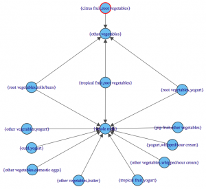
Visualization
The last step is visualization. Lets say you wanted to map out the rules in a graph. We can do that with another library called “arulesViz”.
library(arulesViz) plot(rules,method="graph",interactive=TRUE,shading=NA) |
You will get a nice graph that you can move around to look like this:
References
Resources
![]() Feb 24
Feb 24
Harvesting Tweets with R
Problem Definition

If you are a regular Twitter user, you’ll find yourself wanting to collect all your tweets for whatever obscure reason. I was looking to do some sort of sentiment analysis on a large dataset – it made sense to go to Twitter … but you can only get 1500 tweets at a time with Twitter’s API.
After looking around forums I couldn’t find a reasonable solution. So one way to tackle this is to build up a database over time – just store the tweets you want locally. Since I was going to use this with R, I wanted to collect data with R.
To do this, we can use the twitteR package to communicate with Twitter and save our data.
Once you have the script in place, you can run a cron job to execute the script every day, week, hour or whatever you see fit.
Connecting to Twitter
We will be using 3 libraries in our R Script. Lets load them into our environment:
library(twitteR) library(RCurl) library(ROAuth) |
We will need to set up an SSL certificate (especially if you are on Windows). We do this using the following line of code:
options(RCurlOptions = list(cainfo = system.file("CurlSSL", "cacert.pem", package = "RCurl"))) |
Lets set up our API variables to connect to twitter.
reqURL <- "https://api.twitter.com/oauth/request_token" accessURL <- "https://api.twitter.com/oauth/access_token" authURL <- "http://api.twitter.com/oauth/authorize" |
You will need to get a api key and api secret from Twitter’s developer site https://apps.twitter.com/app/new – make sure you give read, write, and direct message permissions to your newly created application.
apiKey <- "YOUR-KEY" apiSecret <- "YOUR-SECRET" |
Lets put everything together and try an authorize our application.
twitCred <- OAuthFactory$new( consumerKey=apiKey, consumerSecret=apiSecret, requestURL=reqURL, accessURL=accessURL, authURL=authURL) |
Now lets connect by doing a handshake …
twitCred$handshake() |
You will get a message to follow a link and get a confirmation code to input into your R console. The message will look like this:
To enable the connection, please direct your web browser to: http://api.twitter.com/oauth/authorize?oauth_token=4Ybnjkljkljlst5cvO5t3nqd8bhhGqTL3nQ When complete, record the PIN given to you and provide it here:
Now we can save our credentials for next time!
registerTwitterOAuth(twitCred) save(list="twitCred", file="credentials") |
Harvesting Tweets
Now that we are connected we can put in our queries:
- We will use a comma separated string of key words we want to track.
- Once we define our string of key words, we split the string and make a list.
- We will also need a variable to hold our tweets.
I chose key words related to Kuwait.
query <- "kuwaiti,kuwait,#kuwait,#q8" query <- unlist(strsplit(query,",")) tweets = list() |
Now we are ready to ask Twitter for tweets on our key words. What we do in the following block of code is loop through our string of key words; in this case we loop 4 times for our 4 key words.
We use twitteR’s function searchTwitter() which takes the query as a parameter. We also supply additional parameters: n – the number of tweets, geocode – a latitude, longitude and radius (in our example we use within an 80 mile radius of Kuwait City).
for(i in 1:length(query)){ result<-searchTwitter(query[i],n=1500,geocode='29.3454657,47.9969453,80mi') tweets <- c(tweets,result) tweets <- unique(tweets) } |
That’s it, we have our data. All that needs to be done now is save it.
R does not allow you to append data to CSV files, so what we will do is:
- Check if there is a file called tweets.csv and read the data in there
- Merge the data already in the CSV file with our new data
- Remove any duplicates in the data
- Save the file as tweets.csv again
# Create a placeholder for the file file<-NULL # Check if tweets.csv exists if (file.exists("tweets.csv")){file<- read.csv("tweets.csv")} # Merge the data in the file with our new tweets df <- do.call("rbind", lapply(tweets, as.data.frame)) df<-rbind(df,file) # Remove duplicates df <- df[!duplicated(df[c("id")]),] # Save write.csv(df,file="tweets.csv",row.names=FALSE) |
Code
For your convenience, the code in one block:
# Load libraries library(twitteR) library(RCurl) library(ROAuth) # SSL Certificate options(RCurlOptions = list(cainfo = system.file("CurlSSL", "cacert.pem", package = "RCurl"))) # API URLs reqURL <- "https://api.twitter.com/oauth/request_token" accessURL <- "https://api.twitter.com/oauth/access_token" authURL <- "http://api.twitter.com/oauth/authorize" # API Keys from https://apps.twitter.com/app/new apiKey <- "YOUR-KEY" apiSecret <- "YOUR-SECRET" # Connect to Twitter to get credentials twitCred <- OAuthFactory$new( consumerKey=apiKey, consumerSecret=apiSecret, requestURL=reqURL, accessURL=accessURL, authURL=authURL) # Twitter Handshake - you will need to get the PIN after this twitCred$handshake() # Optionally save credentials for later registerTwitterOAuth(twitCred) save(list="twitCred", file="credentials") # Set up the query query <- "kuwaiti,kuwait,#kuwait,#q8" query <- unlist(strsplit(query,",")) tweets = list() # Loop through the keywords and store results for(i in 1:length(query)){ result<-searchTwitter(query[i],n=1500,geocode='29.3454657,47.9969453,80mi') tweets <- c(tweets,result) tweets <- unique(tweets) } # Create a placeholder for the file file<-NULL # Check if tweets.csv exists if (file.exists("tweets.csv")){file<- read.csv("tweets.csv")} # Merge the data in the file with our new tweets df <- do.call("rbind", lapply(tweets, as.data.frame)) df<-rbind(df,file) # Remove duplicates df <- df[!duplicated(df[c("id")]),] # Save write.csv(df,file="tweets.csv",row.names=FALSE) # Done! |
![]() Oct 10
Oct 10
Searching an Excel Sheet with JavaScript
This took some significant amount of time to put together when it really shouldn’t have. Sharing the code here to save anyone else the trouble.
Objective
We will be trying to set up an HTML page that allows users to input a search phrase and trigger a search through an Excel sheet with data.
Approach
- Set up the excel file
- Set up the HTML page with the search field
- Set up the Javascript code
The Excel File
Create an Excel file and fill in column A with values of your choice. Save the file as “example.xls” in your local C:\ folder.
Setting up the HTML Page
Create an html file and open it in your favourite text editor; e.g. “index.html”.
In your text editor create an input field:
<input type="text" name="searchPhrase" />

<a href="javascript: searchExcel();">Search</a>

<div id="results"></div>
The first line creates the input box with the name “searchPhrase”, and the second creates a link that triggers our JavasScript with the function searchExcel. Results will be displayed in the division labelled “results”.
The JavaScript Function
function searchExcel()
{
	var searchPhrase = document.getElementById('searchPhrase').value;
	var Worksheet = 'C:\\example.xls';
	var Excel = new ActiveXObject('Excel.Application');

	Excel.Visible = false;
	var Excel_file = Excel.Workbooks.Open(Worksheet, null, true, null,
        "abc", null, true, null, null, false, false, null, null, null);

	var range = Excel_file.ActiveSheet.Range('A:A');
	var jsRangeArray = new VBArray(range.Value).toArray();

	var found = false;
	for(cells in jsRangeArray)
	{
		if(jsRangeArray[cells] == searchPhrase)
		{
		   document.getElementById("results").innerHTML = "Found";
		   found = true;
		}
	}

	if(found == false)
	{
	    document.getElementById("results").innerHTML = "Not Found";
	}

	Excel.ActiveWorkbook.Close(true);
	Excel.Application.Quit();
	Excel = null;
}
The code is pretty simple really. We’ll go line by line:
- First the value in the input field labelled “searchPhrase” is retrieved.
- The worksheet path is defined as “C:\\example.xls” – the double slash is crucial.
- A new ActiveX object is created – the Excel Application.
- The Excel object is marked as not visible.
- The Excel workbook is opened into the variable Excel_file – you can look up the function definition here on MSDN.
- The range is defined as all cells in column “A” – denoted by Range(‘A:A’);
- The results of the cells extracted are converted into an Arraya that we will use as variable jsRangeArray.
- A new variable “found” is set up to trigger a true or false result for the search.
- We then loop through the Array matching values in the Arraya with the search term.
- If the searchPhrase value matches a value in the Array, the found variable is marked as true and the “results” div is transformed to show “Found”.
- If the loop ends and nothing is found, the “results” div is transformed to show “Not Found”.
- The excel book and the ActiveX object are then closed.
![]() Dec 29
Dec 29
Modifying WordPress RSS Feed
Changing the WordPress RSS is one of the most arduous tasks ever … unless you know how to use hooks.
Hooks are basically functions that do something to an existing process.
Think about it this way, if you were making a cup of coffee, a hook would be sugar that makes a bitter tasting beverage sweet!
The problem: we needed to add a thumbnail to an RSS feed without modifying the wordpress core files.
The solution: create a hook, that modifies the content of each RSS post, before the feed published, and adds in a thumbnail, without affecting the actual post itself.
Here is a zip file containing 2 functions and the hook; fully commented: wpRssEdit.zip
Simply copy and paste this into your theme’s functions.php and it will start working as soon as you update a post or add a new post!
If you want to modify what is added to your RSS feed (say you don’t want a thumbnail, you just want to add a piece of text), just change what the feedContentFilter() does :]
If you need any help, leave a comment ;]
![]() Dec 28
Dec 28
WordPress Get Recent Comments Function
A friend asked me to put up recent comments on http://www.7achy.com
You could use a plugin, but writing your own function gives you a lot more control.
Here is a function called getRecentComments [surprise surprise!] that puts out basic information about recent comments in an unordered list.
Copy and paste the function into your theme’s function.php then call it like this:
getRecentComments(10);
Replace the number with as many comments as you want.
This function is verified and used on this website (bottom right) and soon on http://www.7achy.com
You can edit this function to output a lot more than what’s in there; refer to WordPress’s codex.Then edit the $commentReturn string to include whatever you want.
The funny thing is, I thought this function didn’t work when I tested it here … then I realised :'( there are no comments on my website!! *I has a sad*
![]() Dec 27
Dec 27
Related Posts WordPress Function
Ever wanted to know how you can generate related posts with a function?
Here’s the code for a related posts based on tags and categories; fully commented.
Copy and paste the function into your theme’s functions.php then call it in your loop or anywhere else like this:
echo getRelatedPosts($postID);
Replace $postID with the post ID of the post you want; or use the_ID(); in the loop.
This is verified and used on http://www.q8pd.com
If you want to know more, leave a comment and ask! Enjoy!

